🚀 Motivations
-
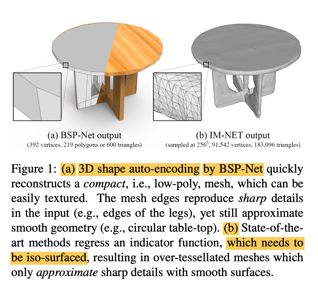
Polygonal meshes are ubiquious in the digital 3D domain,
yet a minor role in deep learning revolution. -
Leading methods for learning genrative models of shapes
rely on implicit functions,
and generate meshes only after
expensive iso-surfacing routines. -
✅ To overcome these challenges,
paper is inspired by a classical spatial data structure from computer graphics,
Binary Space Paritioning(BSP),
to facilitate 3D learning. -
Core ingredient of BSP
is an operation for
recursive subdivision of space
to obtain convex sets. -
By expoliting this property,
paper devised BSP-Net, a network that
learns to represent a 3D shape
vic convex decomposition. -
Convexes inferred by BSP-Net
can be easilty extracted to form a polygon mesh,
without any need for iso-surfacing. -
✅ In this paper, a genearative neural network is develooped
which outputs polygonal meshes.
Paeameters or weights learned by the network
can perdict multiple planes
which fit the surfaces of 3D shape,
resulting in a compact and watertight polygonal mesh. -
🔑 Key Contributions
-
BSP-Net is the fist deep generative network
which directly outputs compact and watertight polygonal meshes
with arbitrary topology and structure variety. -
The learned BSP-tree allows us
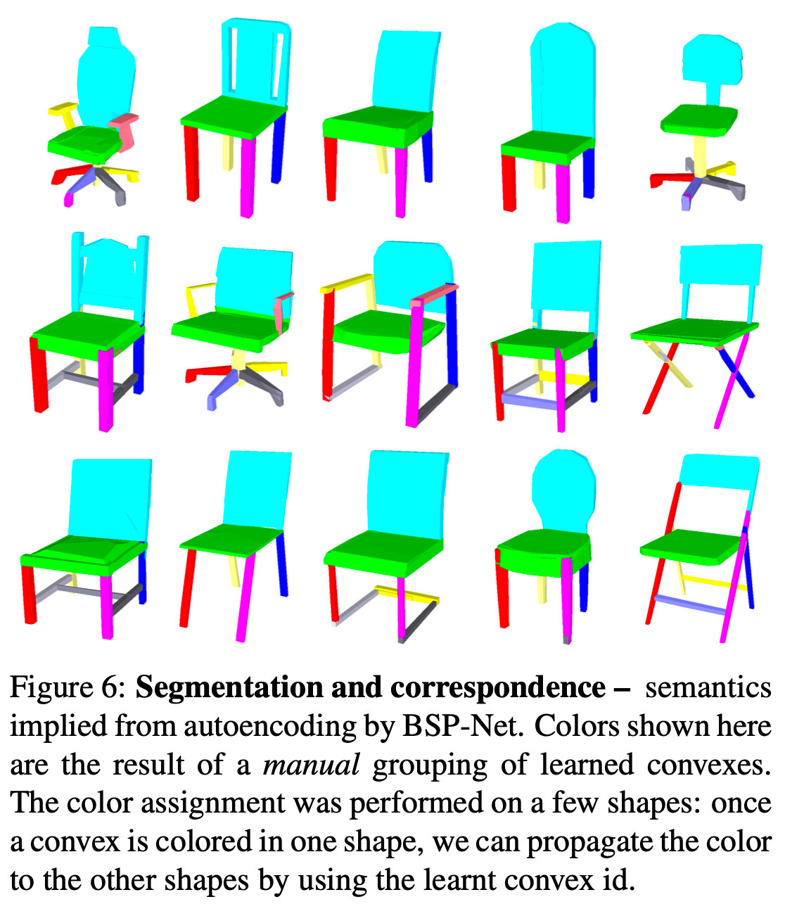
to infer both shape segmentation and part correspondence. -
By adjusting the encode of paper's network,
BSP-Net can be adapted for shape auto-encoding
and single-view 3D reconstruction(SVR). -
BSP-NET is the first to achieve structured SVR,
reconstructing a segmented 3D shpae
from a single unstructured object image.
⭐ Methods
-
BSP-Net learns an implicit field:
input: n point coordinates & shape feature vector
output: value indicating inside or outside the shape -
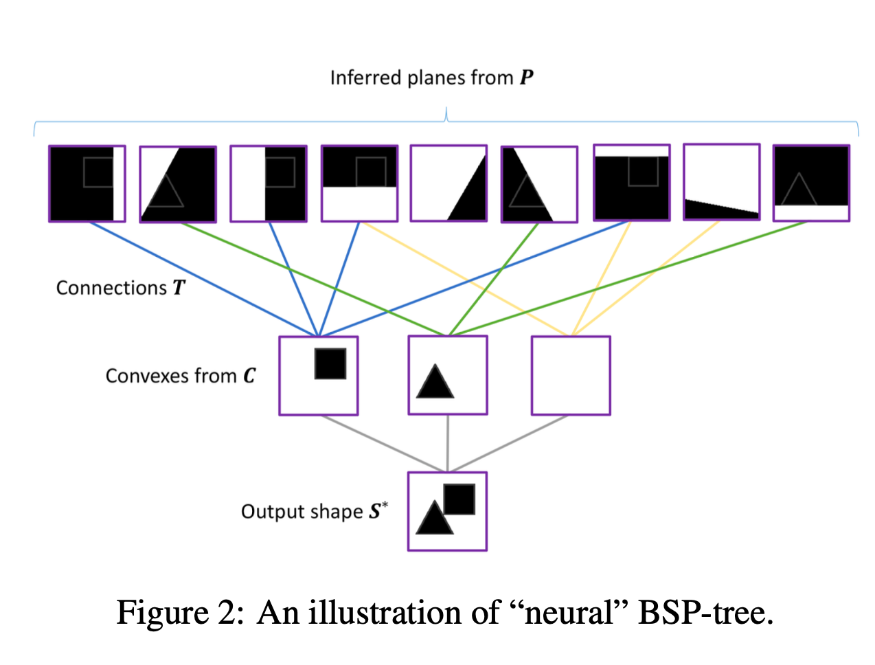
construction of implicit function is illustrated in Fig 2,
and consists of 3 steps. -
1) a collection of plane equations implies
a collection of p binary partitions of space -
2) Operator T(pxc) groups these partitions
to create ca coolection of c convex shape parts -
3) Finally, the part collection is merged
to produce the implicit field of the output shape. -
-
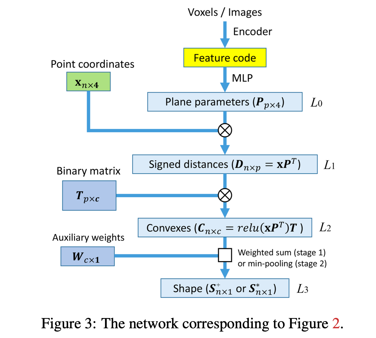
BSP-Net architecture,
corresponding to 3 steps. -
-
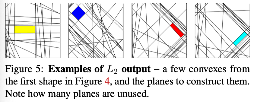
Layer 1) Hyperplane extraction
L0: Input: Feature code,
MLP produces a matrix P(px4) of canonical parameters (plane parameters)
that define the implicit equations of p planes
: ax + by + cz + d = 0
L1: For any point x = (x, y, z, 1),
the product D = xP^T is a vector of signed distances to each plane
(the ith distance is - if x is inside, + if outdise, the ith plane,
w.r.t plane noraml) -
Layer 2) Hyperplane grouping
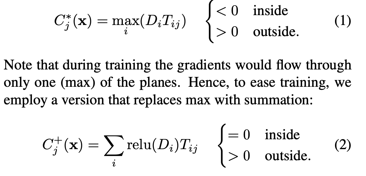
L2: To group hyperplanes into geometric primitives,
paper employs a binary matrix T(px).
Via max-pooling, aggregate input planes
to form a set of c convex primitives
-
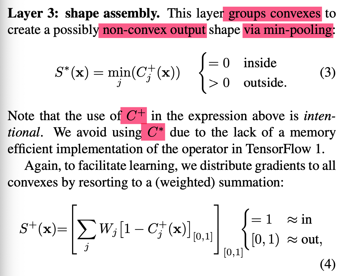
Layer 3) Shape assembly
L3: Finally, assembles the parts into a shape
via either sum or min-pooling.
- At inference time,
feed the input to the network
to obtain components of the BSP-tree,
i.e, leaf node (planes P) & connections (binary weights T)
➡️ Then apply classic CSG(Constructive Solid Geometry)
to extract the explicit polygonal surfaces of the shapes.
Two-stage training
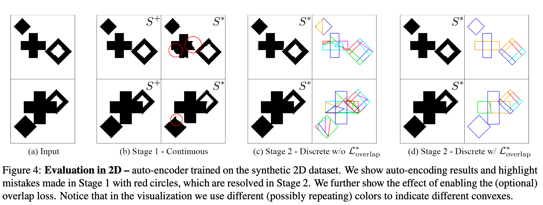
Stage 1: Continuous phase
-
try to keep all weights continuous
and compute an approximate solution vix S+(x)
➡️ Would generate an approximate results (Fig4.b) -
Initialize T & W
with random zero-mean Gaussian noise having σ = 0.02 -
Optimize the network via:

-

Given query points x,
network is trained to match S(x)
to the GT indicator fuction, denoted by F(x|G),
in a least-sqaures sense.
(w~G: sampling specific to the training shape G) -
Continuous relaxation of a graph adjacency matrix T,
where its values are required
to be bounded in the [0, 1] range:

-
Wolud like to W to be close 1
so that the merge operation is a sum:

Stage2: Discreate phase
-
quantize the weights
and use a perfect union
to generage accurate results by fine-tuning on S*(x)
➡️ Would create a much finer reconstruction (Fig4.c,d) -
Quantize T
by picking threshold λ = 0.01
and assign t = (t>λ)?1:0 -
Experimentally paper found the values
learnt for T to be small,
which led to choice of a small threshold value. -
With the quantized T,
fine-tune the network by:

-

This loss function pulls
S(x) towards 0 if x should be inside the shape;
it pushes S(x) beond 1 other wise. -
Optionally, discouraging overlaps between convexes are possible .
First compute a mask M
such that M(x, j) = 1 if x is in convex j
and x in contained in more than one convex, then evaluate:

👨🏻🔬 Experimental Results
Auto-encoding 2D shapes
-
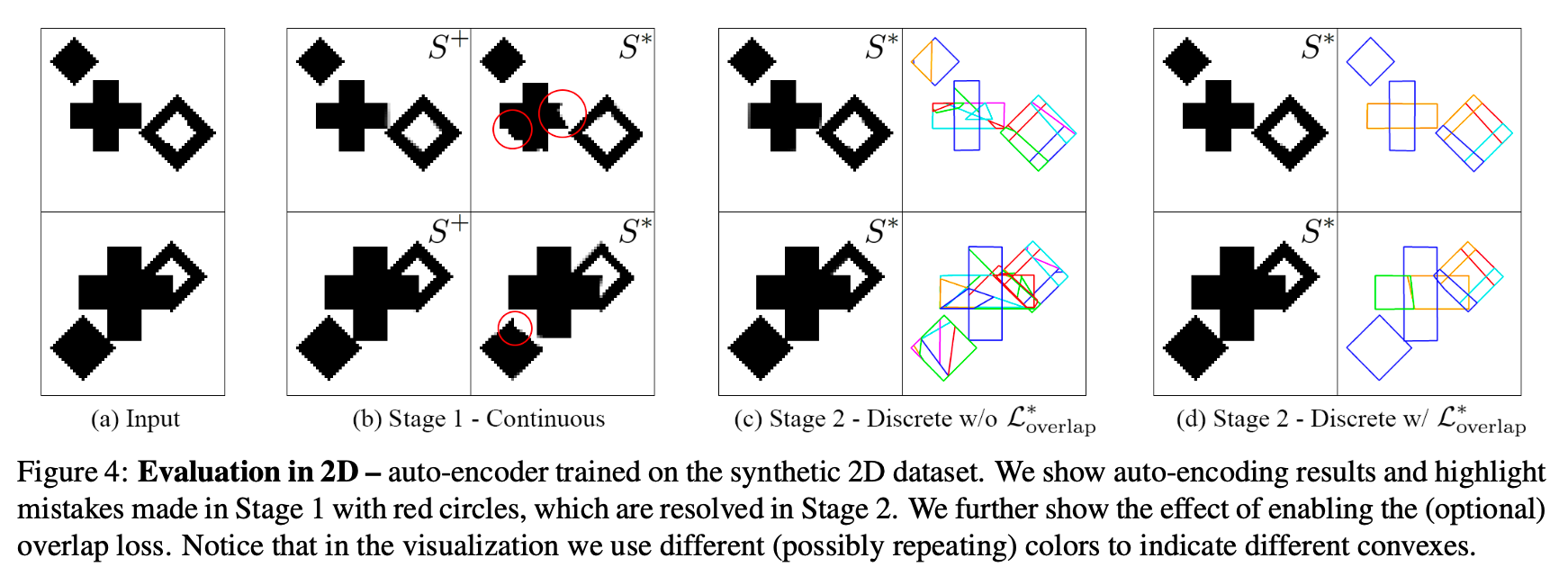
To illustrate how BSP-Net works,
paper created a synthetic 2D dataset.
(diamond, a cross are placed with varying sizes over 64 x 64 images, Fig4.a)
-
After training Stage 1,
network has achieved a good approximage S+ reconstruction,
however, by inspecting S*,
the output of inference have several imperfections -
After the fine-tuning in Stage 2,
network achieves near perfect reconstructions. -
Finally, the use of overlap losses
significantly improves the compactness of representation,
reducing the number of convexes per part (Fig4.d) -
Auto-encoding 3D shapes
-
Dataset: ShapeNet (Part) Dataset
-
Comparison networks:
Volumetric Primitives(VP), Super Quadrices(SP), Branched Auto Encoders(BAE)
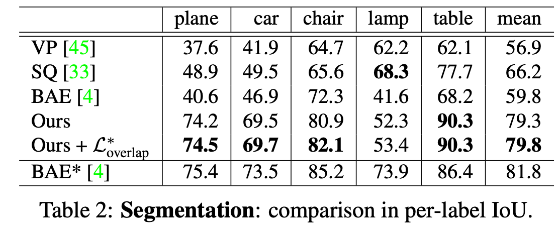
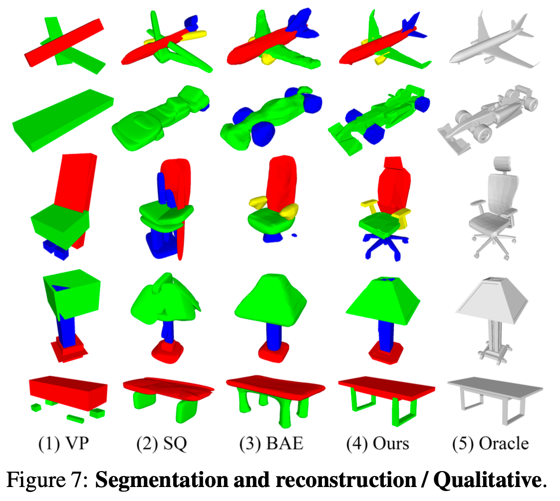
Segmentation
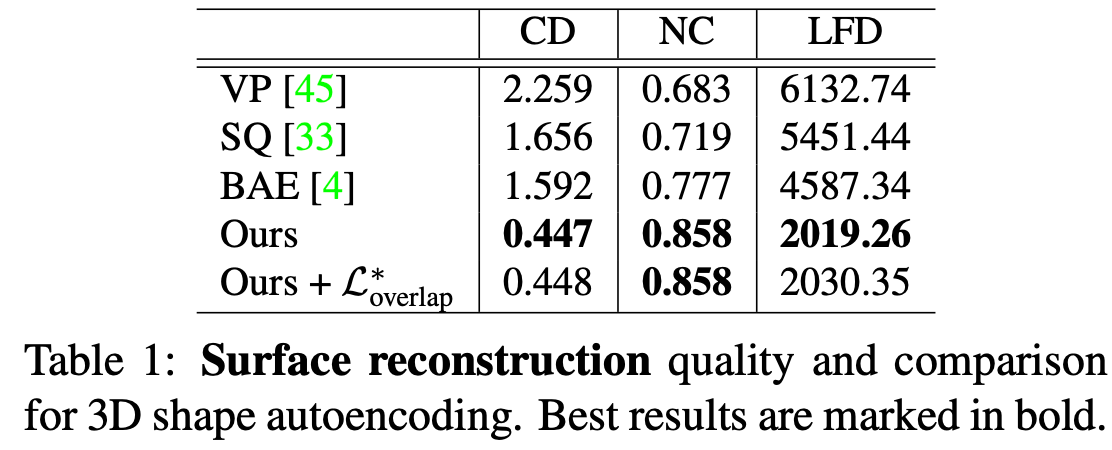
Reconstruction
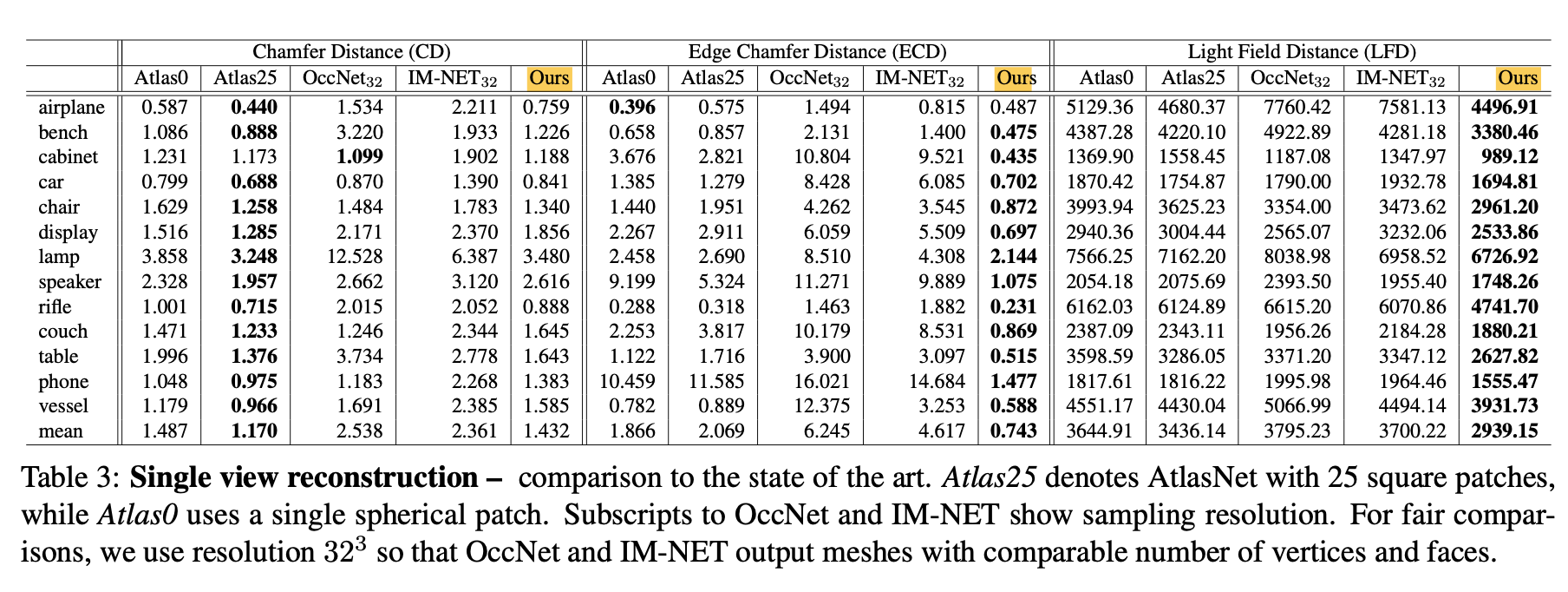
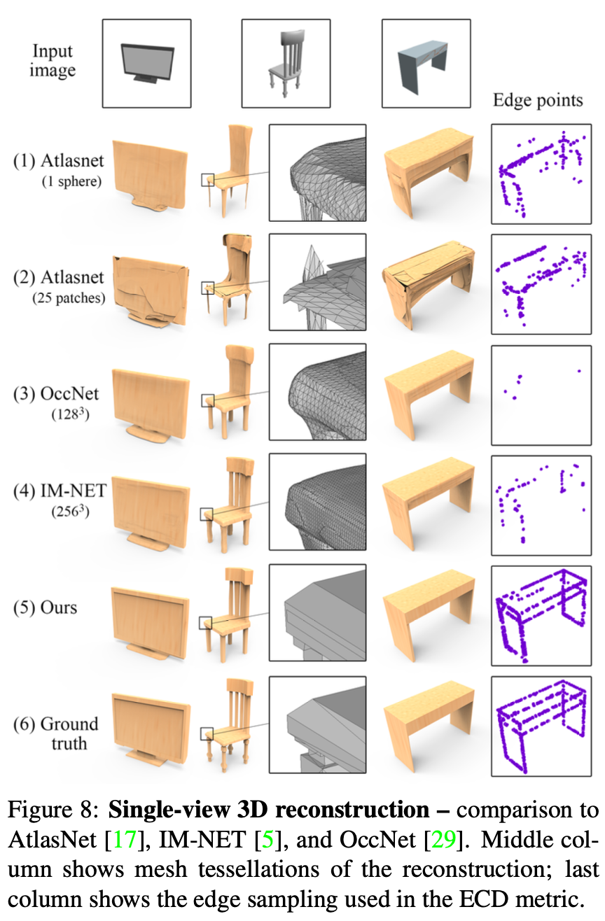
Single view reconstruction (SVR)
-
Dataset: ShapeNet
-
Comparison method:
AtlasNet, IM-NET, OccNet -
-
🤔 Limitation
-
BSP-Net can only decompose a shape as a union of convexes.
Concave shapes, e.g., a teacup or ring,
have to be decomposed into many small convex pieces,
which is unnatural and leads to wasing of a considerable amount of representation budget. -
Training times for BSP0Net are quite significant:
6 days for 4,096 planes and 256 convexes for the SVR task trained across all categories.
✅ Conclusion
-
Paper introudces BSP-Net,
an unsupervised method
which can generate compact and structured polygonal meshes
in the form of convex decomposition. -
Network learns a BSP-tree built on the same set of planes,
in turn, the same set of convexes,
to minimize a reconstruction loss for the training shapes. -
These planes and convexes are defined by weights learned by the network
-
Compared to SOTA methods,
meshes generated by BSP-Net exhibit superior visual qualtiy,
in particular, sharp geometric details,
when comparable number of primitives are employed.
