🚀 Motivations
- Existing categories for 3D representations (voxel, polygon meshes, point clouds) all suffer from different drawbacks and present differenet disadvantages.

🔑 Key Contribution
-
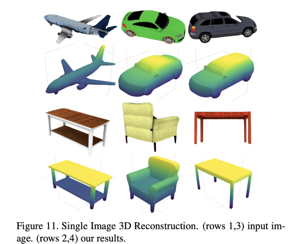
This paper presents a new method for 3D shape reconstruction from a single image, in which a deep neural network directly maps an image to a vector of network weights.
-
The network parametrized by these weights represents a 3D shape by classifying every point in the volume as either within or outside the shape.
⭐ Methods
-
Every shape is represented as a deep NN classifier g, which takes as input points in 3D space.
-
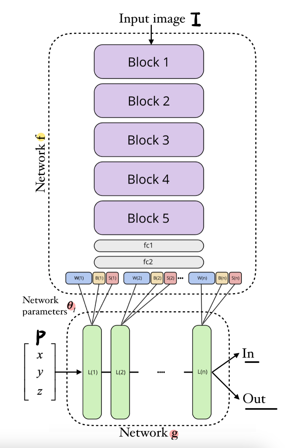
Parameters (weights) of the network g are inferred from the input image, by another network f.
-
Uses a single and straightforward loss.
Consisting Networks
-
Employs two networks f, g with parameter values θf, θI respectively.
-
The networks weights θf are fixed in the model and are learned during the training phase.
-
The weights of network g are a function of input image I, given as the output of the network f.
-
The two networks represent different levels of the shape abstraction.
➡️ f is a mapping from the input image I to the parameters θI of network g,
➡️ g is a classification function that maps a point p with coordinates (x, y, z) in 3D into a score s^pI ∈ [0,1], such that the shape is defined by the classifier'sdecision boundary.

- Parameterize f(I, θf ) as a CNN & g(p, θI) as MLP.
- g(p, θI) should be able to accurately capture both inter and intra shape variations.
Loss Function
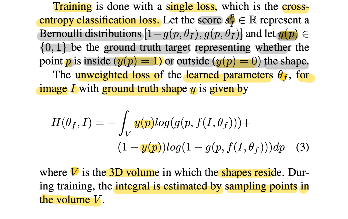
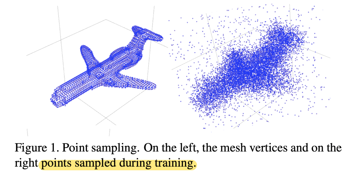
Point sampling during training
- This paper samples more points in the vicinity of the shape's boundary as Points near the decision boundary are more informative.
Architecture
-
Network f is a ResNet with five blocks; g is a fully connected.
-
Network g(p, θI) is an MLP which maps points p ∈ R^3 to a scalar field.
-
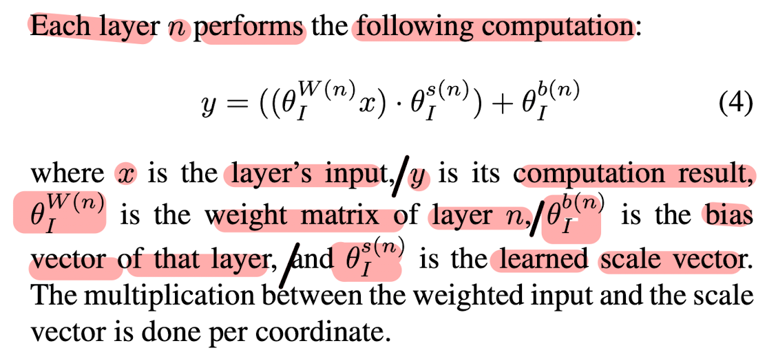
-
ELU activation function is used for the network g
-
Note that the weights of network g are, in fact, feature maps produced by network f, and therefore, represent a space of functions constrained by the architecture of g.
-
f(I, θf ) is a ResNet very similar in structure to the ResNet-34 model.
-
It starts with a convolutional layer that operates on I with N (5 x 5) kernels and then goes through B consecutive blocks.
-
Each block is comprised of 3 residual modules, all utilizing (3 x 3) kernels.
-
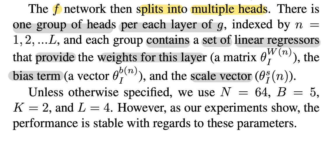
👨🏻🔬 Experimental Results
Training and qualitative results
-
Fig 3 shows the embedding e obtained by the network has learned to esparate between the classes in an unsupervised way.
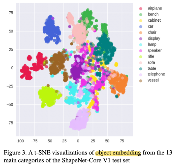
-
Embeddings e1 and e2 obtained from single image I1, I2 of two random shapes from the same class of the test set are linearly interpolated (λe1 + (1-λ)e2) using the interpolation weights λ = 0, 0.25, 0.5, 0.75, and 1 (Fig 4)
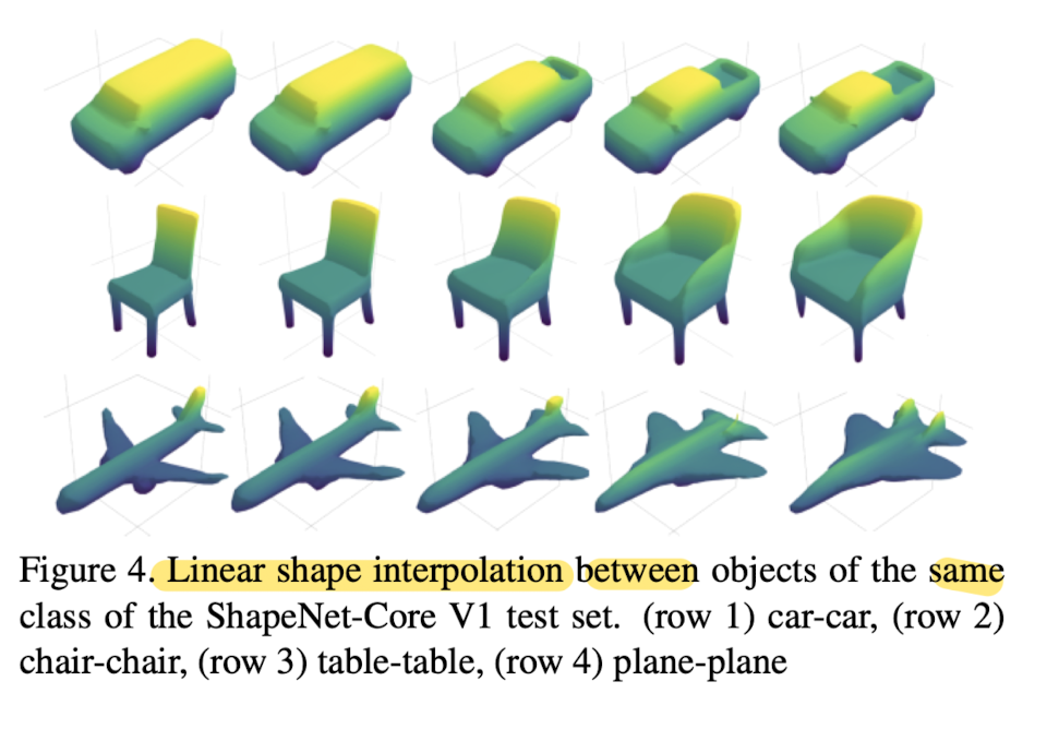
-
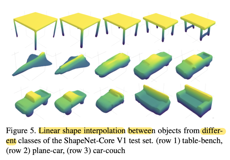
Fig5 shows objects from different classes also blend successfully.
Quantitative results
- 32^3 grid resolution
- Tab2 presents a comparison with the literature methods.

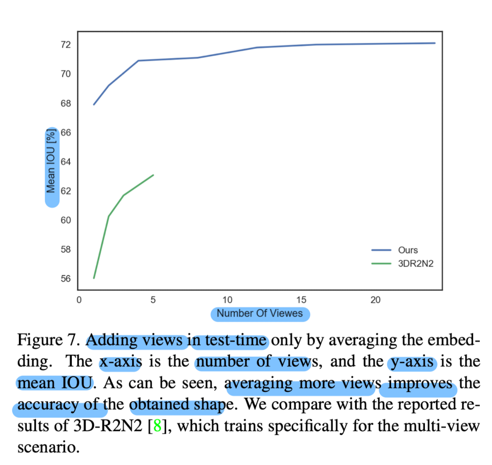
- Performance improves as the number of views increases.
- Multiview results outperform those of 3D-R2N2
Parameter Sensitivity
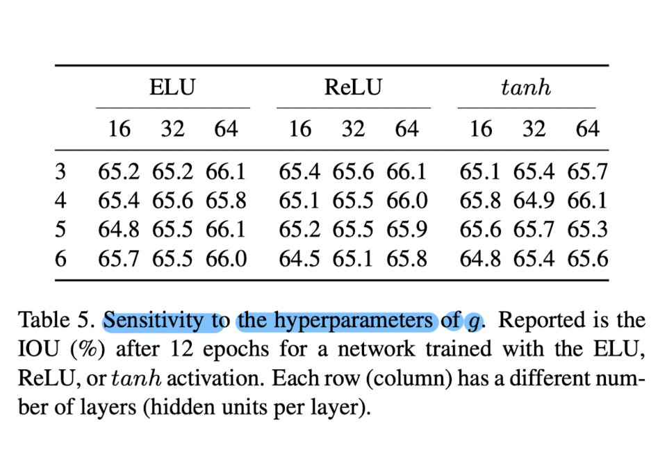
- In Tab.5, This paper evaluated the sensitivity of the method to the architecture of the network g used to represent each shape.
- The performance is relatively constant across the three activation functions tested (ELU, ReLU, and tanh) and for awide range of the number of layers and number of hidden units per layer.
Visualization of Jacobian norm
- This paper evaluates the gradients of G w.r.t p(x,y,z) which correspond to the Jacobian of g.

- Obtained norm can be viewd as a local sensitivity score of the shape.
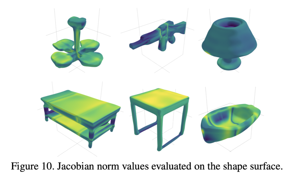
- Low norms are yellow and high norms are bluish.
- Flat surfaces present smaller gradient norms than the highly curved sufaces.
- Note that the direction of the gradient is always normal to the surface, which is a property of isosurfaces.
