🔑 Key Contributions

• This paper presents an end-to-end pipeline for rendering images from novel views with only image supervision that leverages an internal 3D volumetric representation.

• This paper proposes using a volumetric representation consisting of opacity and color at each position in 3D space, where rendering is realized through intergral projection.

• This paper shows that a NN decoder is sufficient to encourage discovery of solutions that generalize across viewpoints.

• This paper employs a warping technique that indirectly escapes the restrictions imposed by a regular grid structure,
  allwoing the learning algorithm to make the best use of avail. memory.

⭐ Methods

• Method has two primary components:
  1) encoder-decoder network ➡️ transforms input images into a 3D volume representation V(x)
  2) Differentiable ray-marching step
  ➡️ renders an image from the volume V given a set of camera parameters.

• The method can be though of as an autoencoder whose final layer is fixed-function(i.e., no free parameters) volume rendering operation.

• This method models a vloume that maps 3D positions x ∈ ℝ^3,
  to a local RGB color and differential opacity at that point.
  

---

• below Fig 2 shows a visual representation of the pipeline.
  

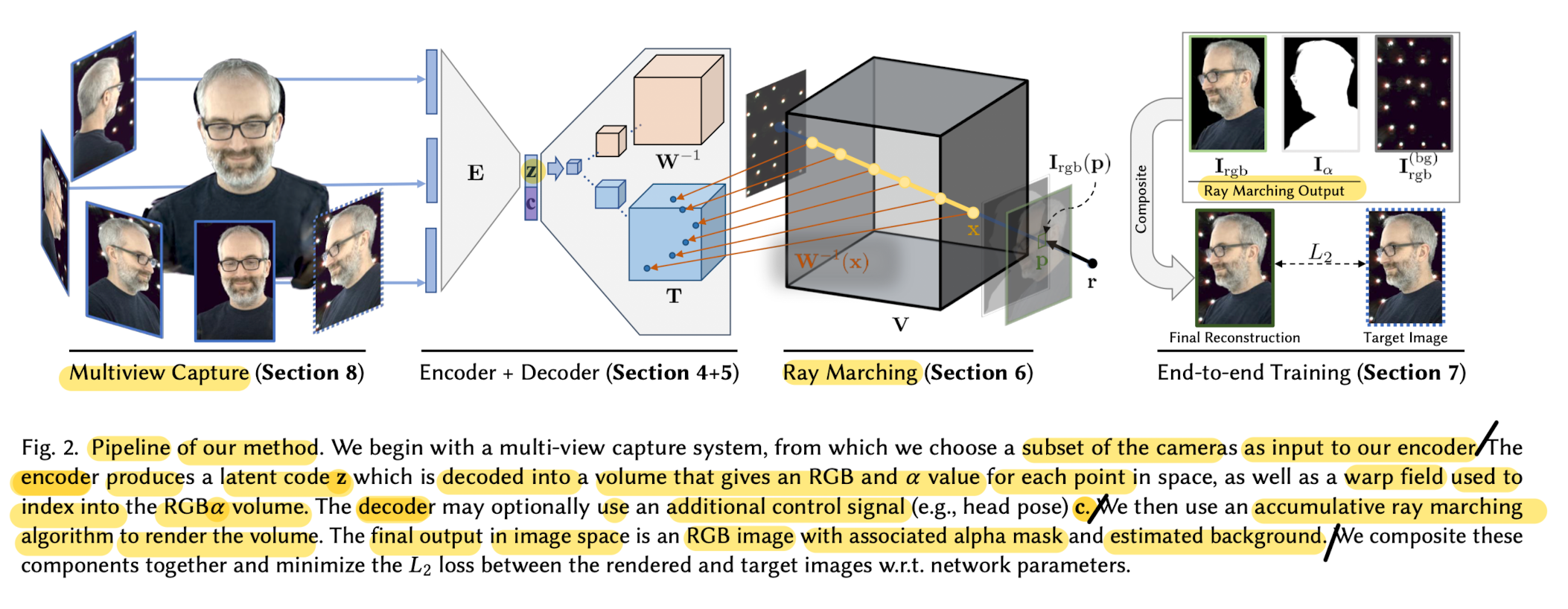
1) Capture a set of synchronized and calibrated video streams of a performance form different viewpoints.

2) Encoder network takes images from a subset of the cameras for each time instant,
and produces a latent code z that represents the state of the scene at that time.

3) Volume decoder network produces a 3D volume given this latent code, V(x;z),
which yields an RGBα value at each point x

4) Accumulative ray marching algorithm renders the volume from a particular point-of-view.

5) Train this system end-to-end by reconstructing each of the input images
and minimizing the squared pixel reconstruction loss over the entire training set.

• At training time, run through the entire pipeline to train the weights of the encoder-decoder network.

• At inference time, produce a stream of latent code z
  (either the sequence of latent codes produced by the training images or a novel generated sequence)
  and decode and render in real time.

ENCODER NETWORK

• The main component that enables novel sequence generation is the encoder-decoder architecture,
  where scene's state is encoded
  using a consistent latent representation z ∈ ℝ^256.

• A traversal in this latent space can be decoded into a novel sequence of vloumes,
  that can then be rendered from any viewpoint.

• To bulid the latent space,
  the information state of the scene at any given time is codified
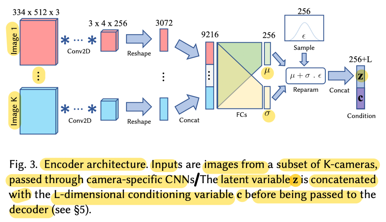
  by encoding a subset of views form multi-camera capture system using a CNN.

• Each camera view is passed through a dedicated branch
  before being concatenated with those from other views
  and further encoded down to the final shape.

• Although using all camera views as input is optimal from an information-theoretic perspective,
  this paper found that using K = 3 views worked well in practice,
  while memory and computationally efficient.

• To maximize covergae,
  paper selects a subset of cameras that are roughly orthogonal,
  alothough this system is not sensitive to the specific choice of views.
  They used frontal, left and right-most camer views.

• To generate plausible samples during a traversal through latent space,
  the generatie model needs to generalize well between training samples.
  This is achieved by learning a smooth latent space.
  ➡️ To encourage smoothness,
  paper uses a variational arch.
  Encoder outputs parameters of a diagonal 256-dimensional Gaussian(i.e., μ and σ),
  whose KL-divergence from a standard Normal distribution is used as regularization.
  ➡️ Generating an instance involves sampling from this distribution uising the reparameterization trick,
  and decoding into the volumetric components.

VOLUME DECODERS

• This section is about parameterizing the RGBα volume function V using differnet NN arch, which are called volume decoders

Possible representations for volumes

1) MLP Decoder

• One possible model for the volume function V(x;z) at point x with state z,
  is an implicit one with a series of fully connected layers with non-linearities

2) Voxel Grid Decoders

• Volume function can be modeled as a discrete 3D grid of voxels.

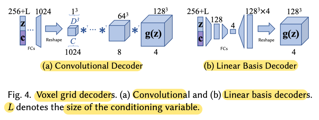
• Produce this explicit 3D voxel grid as the output tensor of a NN.
  

• tensor Y ∈ ℝ^(C x D x D x D)
  represents a D x D x D grid of values in ℝ^C, with C the channel dimensions.

• Define S(x; Y): ℝ^3 -> ℝ^C to be an interpolation function
  that samples from the grid Y
  by scaling continuous values in the range -1 ~ 1
  to the grid 1 ~ D along each dimension,
  followed by trilinear interpolation.

• Define a volume decoder for a 3D cube with
  center at x0, and sides of size W,
  where g(z) is a NN that produces a tensor of size 4 x D x D x D
  (in practice, paper uses either a convolutional arch or a series of fully-connected layers to implement g(z))
  

• After decoding the volume,
  apply a softplus function to the RGBα values
  to ensure they are non-negative.

Warping Fields

• To deal with problems that
  voxel grids are limited in representing details (as small as a singl voxel)
  and computationally expensive to evaluate and store at high resolution

• Paper proposes to use warping fields to both
  the effective resolution of the voxel volumes
  as well as model motion more naturally.

• In warping formulation,produce
  a template RGBα volume T(x) and
  a _warp volum_e W^(-1)(x).

• Each point in the warp volume gives a corresponding location in the template volume from which to sample,
  making this an inverse warp
  as it maps from output positions to template sample locations.

• The choice of inverse warps rather than forward warps
  allows representing resolution-increasing transformations by mapping a small area of voxels in the output space
  to a larger area in the template space
  without requiring additional memory.

• Define inverse warp field
  where x : 3D point in the output(rendering) space
  y : 3D point in the RGBα template space
  

• To generate the final volume value,
  evaluate the value of the inverse warp
  and then sample the template volume T at the warped point.
  

Mixture of Affine Warps

• Paper takes the apporach that the basic building block of a warp filed should be an affine warp.

• Since single affine warp can't model non-linear bending,
  use a spatial mixture of affine warps to produce an inverse warp field.

• Write the affine mixture as
  

• Ai(x): i th affine transformation,
  { Ri, si, ti }: rotation, scaling, and translation of the i th _affine transformation params.
  ◦: element-wise multiplication
  wi(x): weight volume of the i _th warp
  

• In practice, paper founds that a mixture of 16 warps provides sufficient expressiveness

View Conditioning

• In order to model view-dependent appearnce,
  condition the RGB decoder network on the viewpoint.
• Input normalized direction of the camera to the decoder, alongside the encoding

ACCUMULATIVE RAY MARCHING

• Formulate a renderin gprocess for semi-transparent volumes
  that mimics front-to0back additive blending:
  As a camera ray traverses a volume of inhomogeneous material,
  it accumulates color in proportion to the
  local color and density of the material at each point aloing its path.

Semi-Transparent Volume Rendering

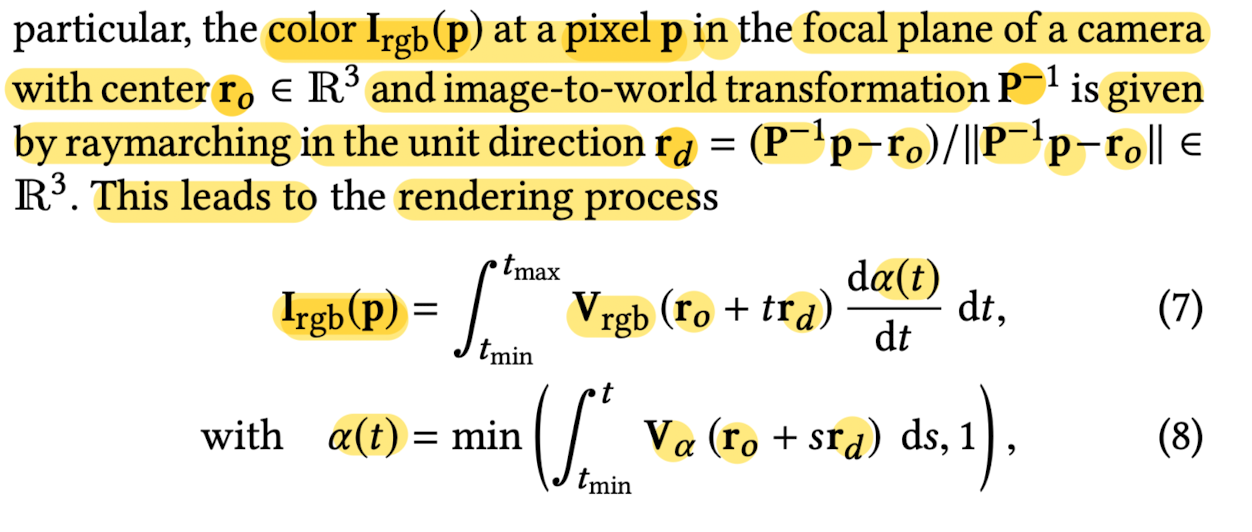
• Paper generates images from a volume function V(x)
  by marching rays through the volume it models.

• To model occlusions,
  the ray accumulates not only color but also opacity.

• If accumulated opacity reaches 1,
  then no further color can be accumulated on the ray.

• 

• 

• 

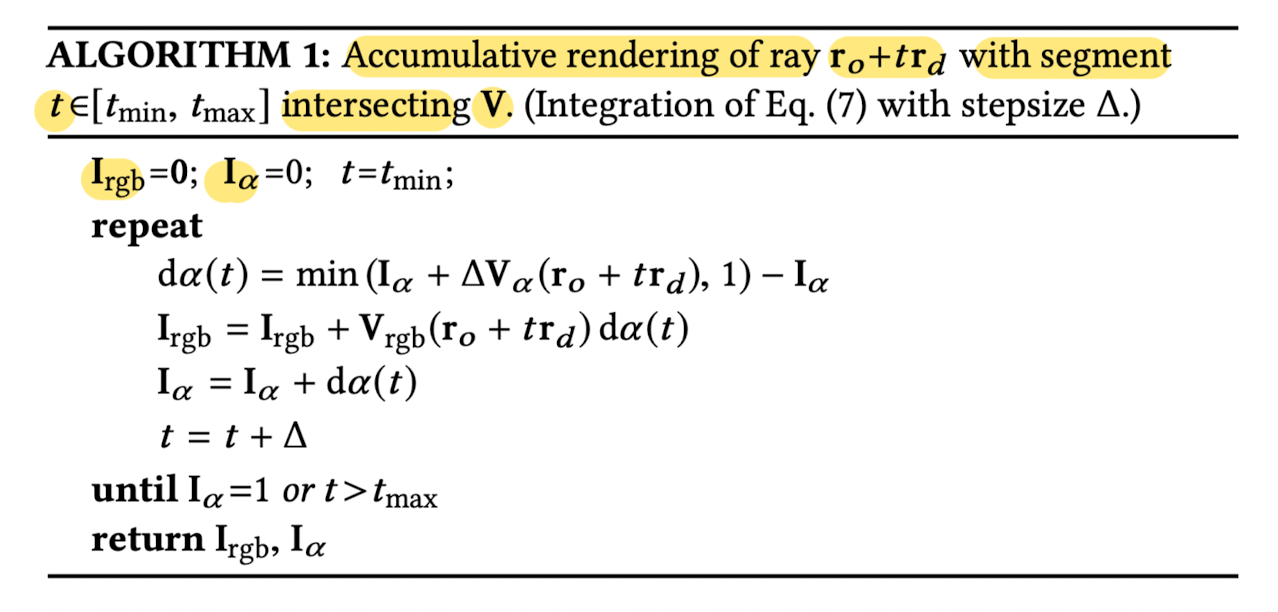
• Algorithm1 shows the computation of the output color
  for a ray intersecting the volume V,
  and represents the unmerical intergrations of Eqs. 7,8
  using the rectangle rule.

• This image formation model is differentiable,
  which allows to optimize the parameters of the volume V
  to match target images.

END-TO-END TRAINING

• Training the system consists of training the weights θ of the encoder-decoder network.

1) Color Calibration

• Introduce a per-camera and per-channel gain g and bias b
  that is applied to reconstructed image before comparing to GT.
• This allows system to account for slight differences in overall intensity in the image.

2) Backgrounds

• To ensure that algorithm only reconstructs the object of interest,
  estimate a per-camera background image
  
• Background image is static across the entire sequence,
  capturing only stationary objects that are generally outside of the reconstruction volume.
• Obtain a final image
  
  from a specific view
  by raymarching all pixels p according to Eq 7
  and merging
  
  with its corresponding background pixel
  
  according to the reamining opacity when exiting the volume,
• 

3) Reconstruction Priors

• Without using priors,
  the reconstructed volumes tend to include smoke-like artifacts.

• These artifacts are caused by slight differences in appearance from different viewpoints
  due to calibration errors or view-dependent effects

• The system can learn to compensate for theses differences
  by adding a small amount of opacity
  that becomes visible from one particular camera.
  

• To reduce these artifacts, introduced two priors:

1. regularizes the total variation of the log voxel opacities
   
   where sum is perfomed over all the voxel centers x
   and N is the number of voxels.
   This term helps recover sharp boundaries between opaque and transparent regions
   by enforcing sparse spatial graidents.
   apply this prior in log space to increase the sensitivitiy of the prior to small α values
   because the artifacts tend to be mostly transparent.

2. beta distribution (Beta(0.5, 0.5)) on the final image opacities Iα(p)
   write regularization term using the negative log-likelihood of the beta distribution,
   

👨🏻‍🔬 Experimental Results

• For all experiments, paper uses the convolutional volume decoder with size 128^3.

Warping Method

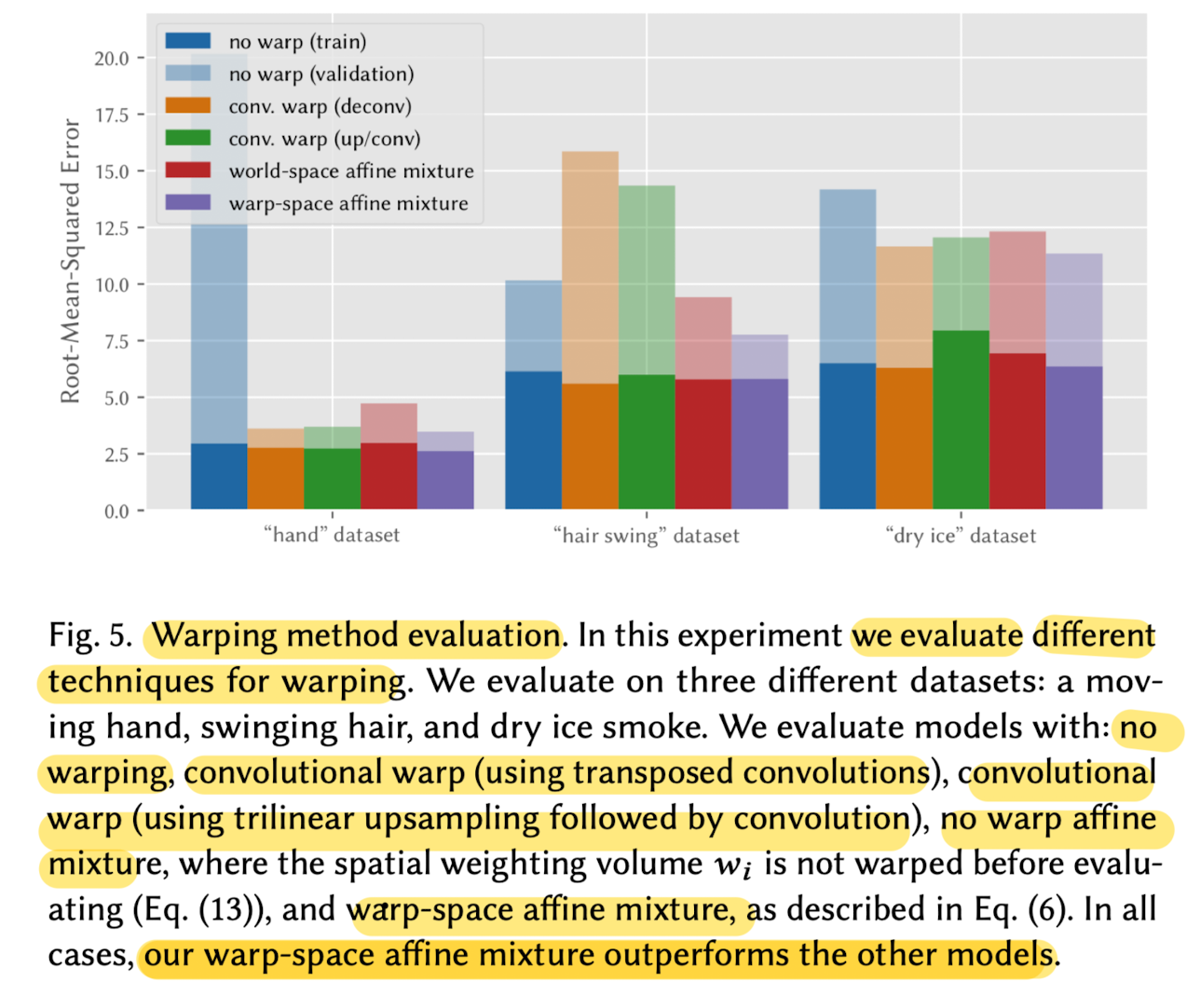
• To validate warp representation,
  compared aginst several variangts
  : model with no warping, model with a warp produced by a CNN,
  a model that doen not apply the warp before computing the affine mixture weight,
  and the proposed affine mixture warp model.

View-Conditioning

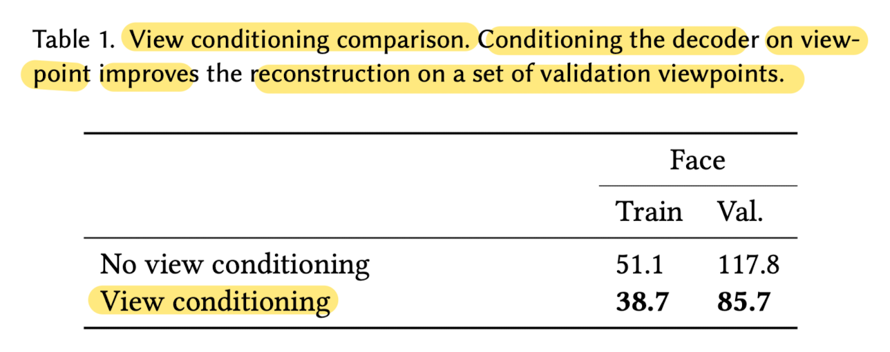
• An important part of rendering is
  being able to model view-dependent effects such as specularities.
• To do this, we can condition the RGB decoder V rgb
  on the viewpoint of the rendered view.
• This allows the network to change the color of certin parts
  of the scene depending on the angle it's viewed from.
  

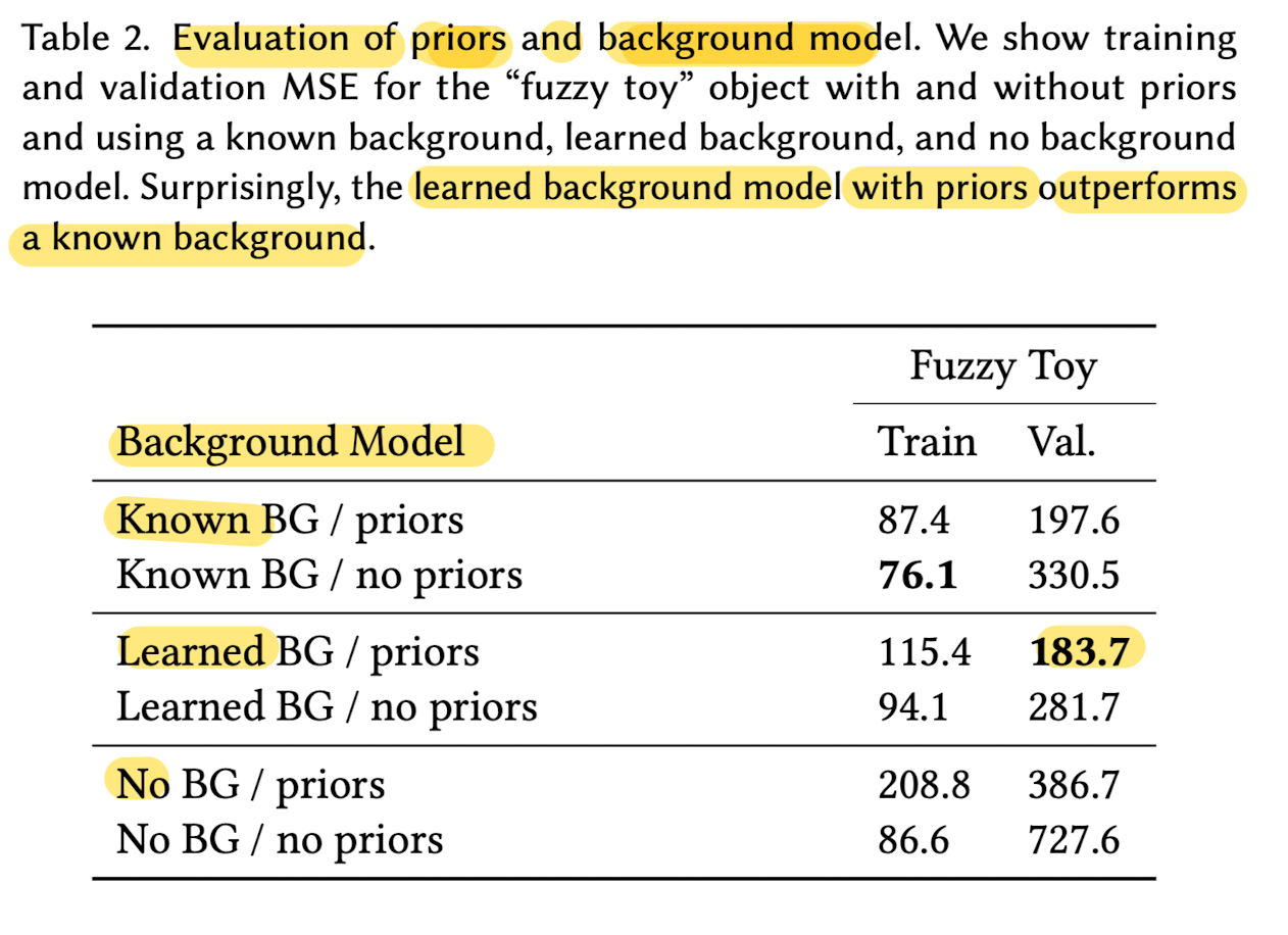
Priors and Background Estimation

• Paper imposed several priors
  on the reconstructed volume
  to help reduce the occurrence of artifacts in reconstruction.

• Paper evaluated the effectiveness of background estimation and the priors
  on the reconstructed volume quality
  in terms of mean-squared-error on the validation viewpoints.

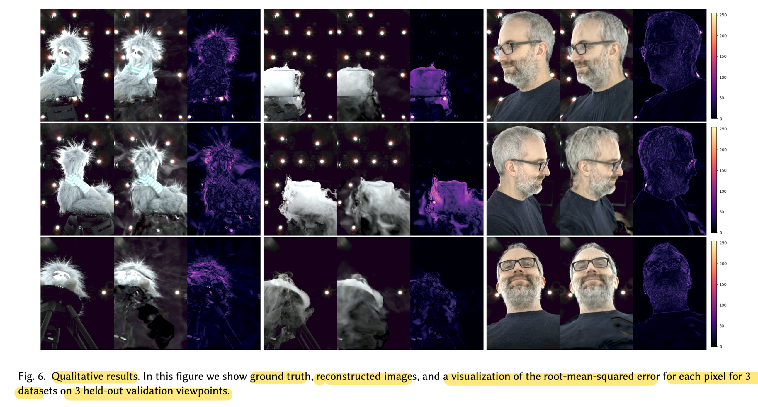
Qualitative Results

• Renderings demonstrate that our method is able to model difficult phenomena like fuzz, smoke, and human skin and hair.

• Figure also shows typical artifacts, produced by reconstructions
  : typically, a very light smokey pattern is added
  which may be modeling view-dependent appearnce for certain training cameras.
  Using more camera views tends to reduce all artifacts.
  

---

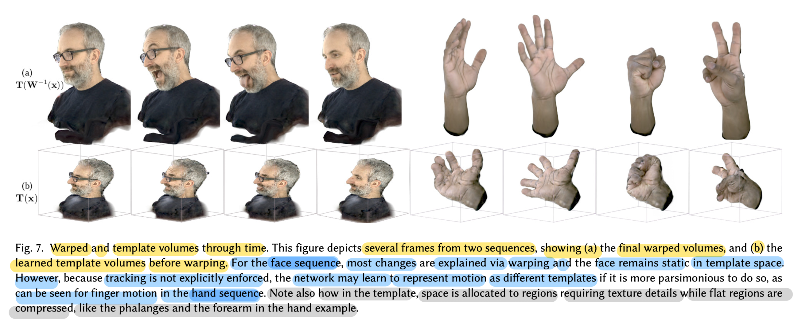
• Fig 7 shows how the template volume changes through time, across several frames,
  compared to the final warped volume that is rendered.

• Ideally, object motion should be represented entirely by the warp field.

• However, this does not always happen
  when representing such changes requires more resolution than is available
  or because representing the warp field becomes too complex.
  

---

• Fig 11 visualizes the learned RGBα volumes.
  While there is no explicit surface reconstruction obejective in paper's method,
  paper can visualize iso surfaces of constant opacity, shown in (b)
  

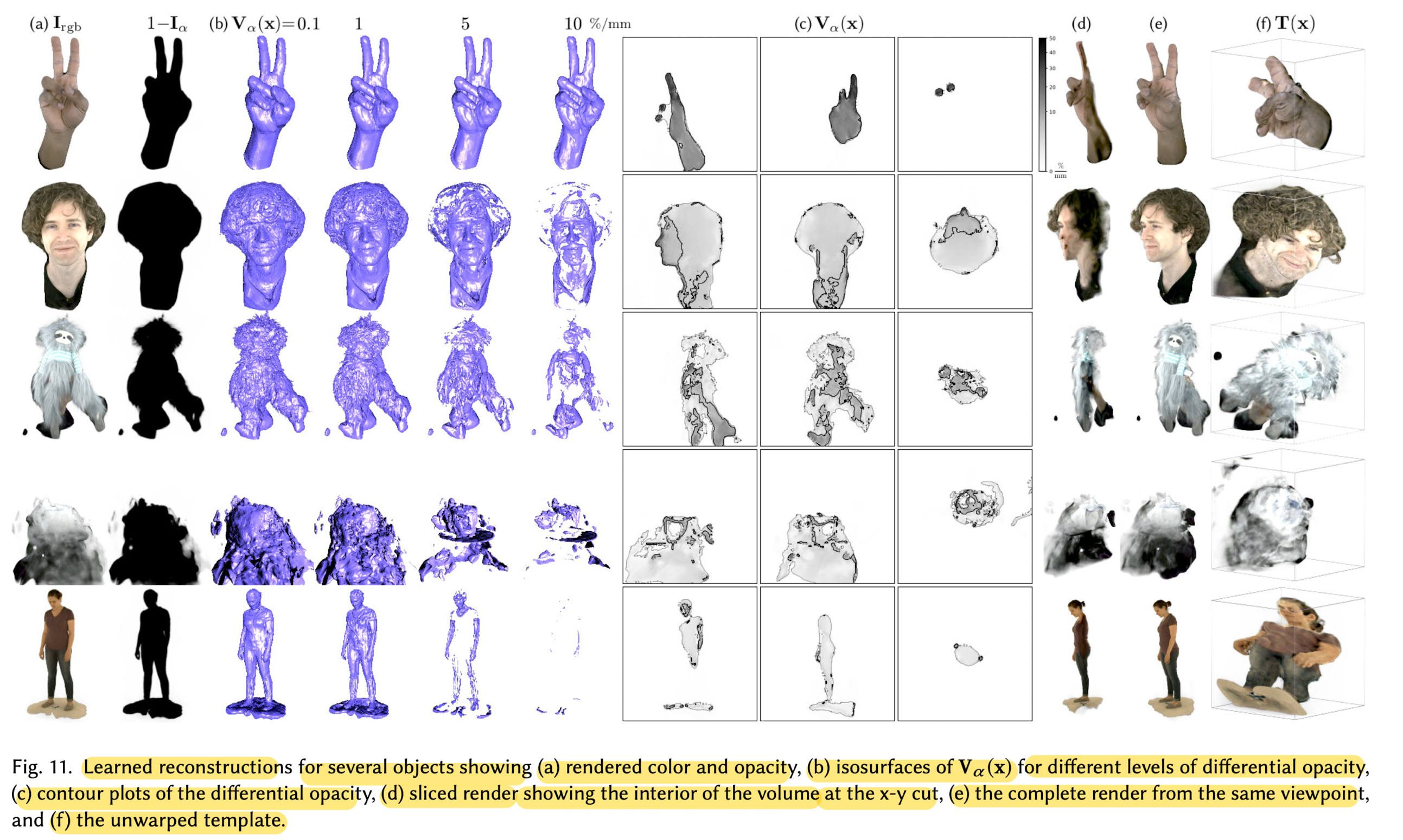
• Ideally, fully opaque surfaces such as the hand in the first row would be represented by delta functions in Vα(x),
  but we find that method trades off some opacity to better match reconstruction error in the training views.

• Note how translucent materials, such as the glasses in the second row,
  or materias which appear translucent at coarse resolution, such as hair in the 3rd and 4th rows,
  are modeled with lower opacity values
  but retain a distnct structure particular to object.

Animating

• Latent variable model alllows to create new sequences of content by modifying the latent variables.

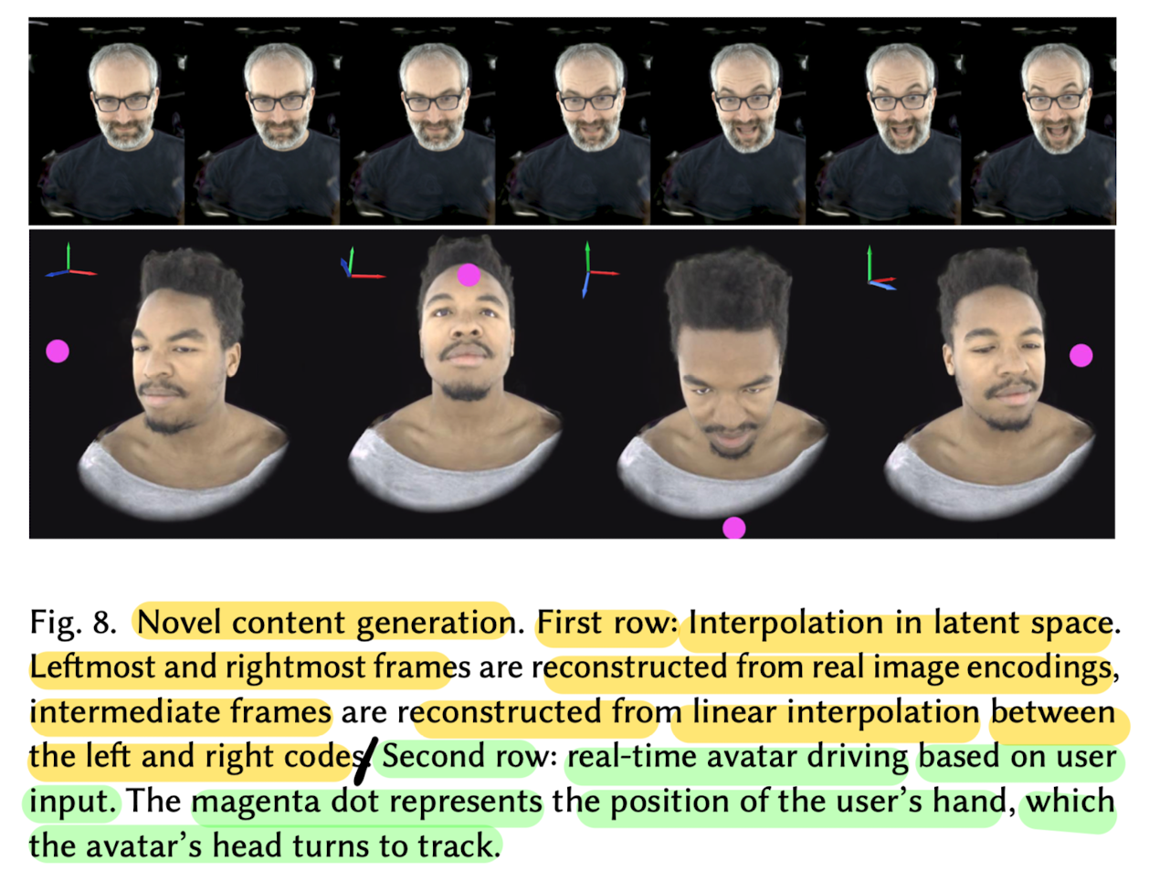
• Fig 8 shows two examples of content modification
  by interpolating leatent codes
  and by chainging the conditioning variable based on user input.

• Latent space interpolation shows that
  the encoder network learns a compact representation of the scene.

• In the seconde example, conditioned the decoder on the head pose of the subject,
  allowing to create novel sequences in real time.
  

---

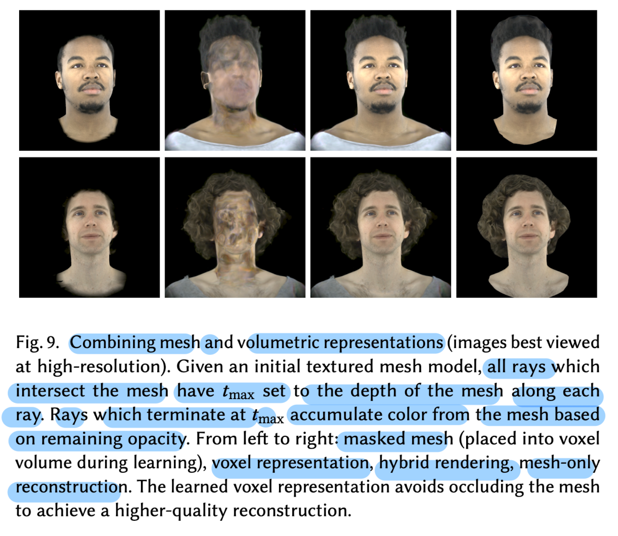
• Fig 9 shows the results of combining a textured mesh represntation with paper's voxel representation.
• Textured meshes can efficiently and accurately represent fine detail in regions of the face like the skin and eyes
• while the voxel representation excels at modeling hair.
  

🤔 Limitations

• Given a surface with limited texture,
  estimead volume may represent that surface as transparent
  and place its color in the background,
  so long as doing so does not cause otherwise occluded surfaces to appear.

• Although method can handle transparent objects, like plastic bottles,
  the method doesn't currently consider refractive surfaces.
  Model can represent dull specular highlights through view conditioning
  but high-frequency specular highlights are not correctly represented.