Pipeline이란?
데이터 전처리부터 모델 학습까지의 과정을 하나로 묶어주는 도구
👉 “데이터 → 스케일링 → 모델 학습” 이 흐름을 줄줄이 이어 붙여서 자동화하는 것
왜 쓰냐면?
- 코드 깔끔해짐
- 실수 줄어듦 (예: 훈련/테스트 데이터에 같은 전처리 적용 안 했을 때)
- GridSearch 등 하이퍼파라미터 튜닝에도 완전 편함
기본 구조
from sklearn.pipeline import Pipeline
from sklearn.preprocessing import StandardScaler
from sklearn.linear_model import LogisticRegression

pipeline = Pipeline([
    ('scaler', StandardScaler()),         # 1단계: 스케일링
    ('model', LogisticRegression())       # 2단계: 모델 학습
])
사용법
pipeline.fit(X_train, y_train)      # 전체 파이프라인 학습
pipeline.predict(X_test)           # 전처리 포함 예측
→ fit하면 scaler도 fit되고, model도 fit됨!
→ predict하면 자동으로 스케일링까지 처리한 다음 예측해줌 👍
파이프라인에 들어갈 수 있는 요소들
| 단계 | 가능 요소 |
|---|---|
| 전처리 | StandardScaler, MinMaxScaler, OneHotEncoder, SimpleImputer 등 |
| 특성 선택 | SelectKBest, PCA, PolynomialFeatures 등 |
| 모델 | LogisticRegression, RandomForestClassifier, SVC, XGBClassifier 등 |
예시: 전처리 + 분류기
from sklearn.pipeline import Pipeline
from sklearn.impute import SimpleImputer
from sklearn.preprocessing import StandardScaler
from sklearn.ensemble import RandomForestClassifier

pipe = Pipeline([
    ('imputer', SimpleImputer()),           # 결측치 처리
    ('scaler', StandardScaler()),           # 스케일 조정
    ('clf', RandomForestClassifier())       # 모델 학습
])

pipe.fit(X_train, y_train)
y_pred = pipe.predict(X_test)
실습
전에 했던 와인 데이터를 갖고 Pipeline을 구현해보자~
전에는 StandardScaler -> split -> DecisionTreeClassifier 생성 -> fit 이런 순으로 했었다면,
from sklearn.pipeline import Pipeline
from sklearn.tree import DecisionTreeClassifier
from sklearn.preprocessing import StandardScaler

estimators = [
    ('scaler', StandardScaler()),
    ('clf', DecisionTreeClassifier())
]

pipe = Pipeline(estimators)
요렇게 간단하게 할 수 있음!
pipe를 찍어보면..
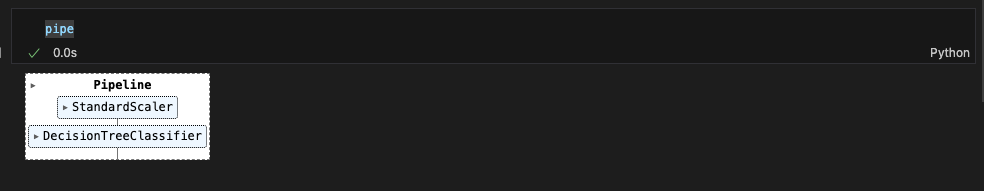
StandardScaler 다음에 DecisionTreeClassifier가 차례로 수행되었구나.
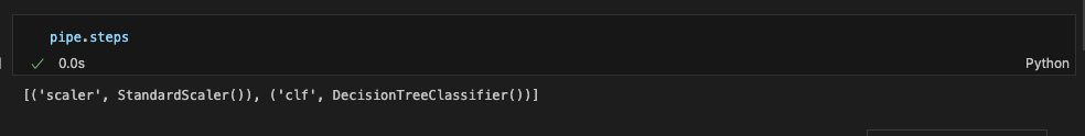
.steps 를 통해서도 확인 가능
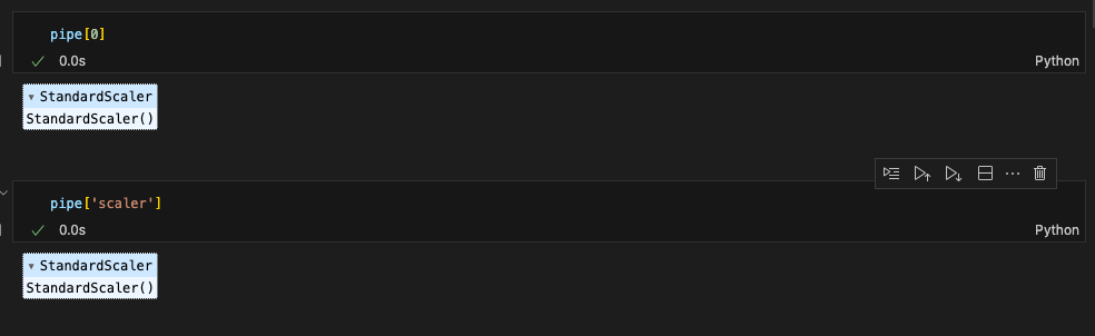
pipe[0] 또는 pipe['scaler'] 이런식으로 스텝별 객체를 호출할 수도 있다.
set_params()를 통해 파라미터값 세팅 가능
(파라미터는 스텝이름__속성이름 이런식이므로 주의 / 언더바 두개!)
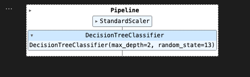
pipe.set_params(clf__max_depth=2)
pipe.set_params(clf__random_state=13)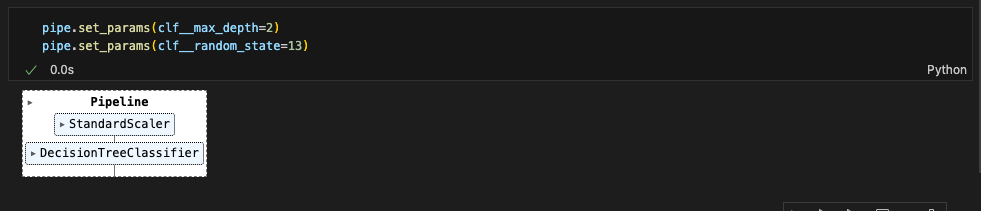
Pipeline을 이용해서 이전에 했던 분류기를 만들어보면!
train/test 데이터 split해준 다음, pipeline으로 fit~
(Pipeline은 데이터 전처리, 모델 학습, 예측의 전체 흐름을 하나로 묶어주는 역할. 학습된 데이터만 사용해서 처리할 수 있도록 설계되어있어서, X_train, X_test, y_train, y_test는 미리 나눠줘야 함)
from sklearn.model_selection import train_test_split

X_train, X_test, y_train, y_test = train_test_split(X, y, test_size=0.2, random_state=13)
pipe.fit(X_train, y_train)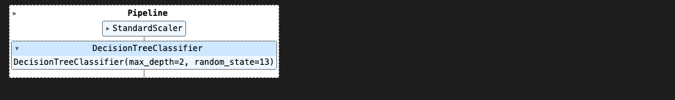
매우 간단해졌다.
성과 확인도 해주기.
from sklearn.metrics import accuracy_score

y_pred_test = pipe.predict(X_test)
accuracy_score(y_test, y_pred_test)
결정 트리 시각화에 많이 쓰이는 graphviz로 결정트리를 시각화해보면,
from graphviz import Source
from sklearn.tree import export_graphviz

Source(export_graphviz(pipe['clf'], feature_names=X.columns,
                       class_names=['W', 'R'],
                       rounded=True, filled=True))
이렇게 모델 구조도 확인할 수 있다.
(이 글은 제로베이스 데이터 취업 스쿨의 강의 자료 일부를 발췌하여 작성되었습니다.)