RL Course by David Silver - Lecture 6: Value Function Approximation

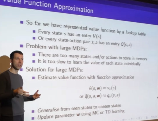
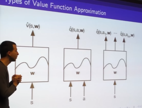
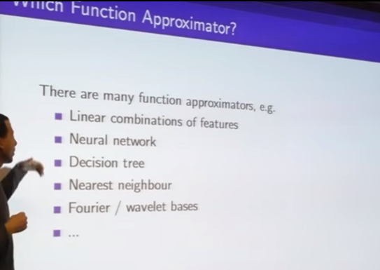
• variable function approximator

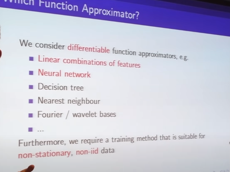
• focus on Linear combinations of features as canonical case
• also non linear combination like Neural network

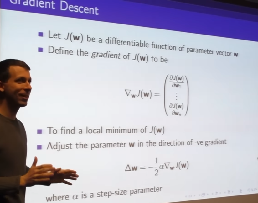
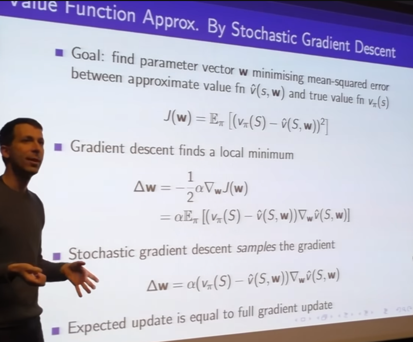
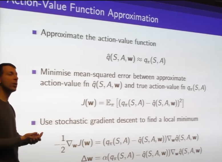
• if we know $v_{\pi}$ we would know the error term easily
• error is target to correct and gradient is how to correct
• minimize 평균 제곱 오차Mean squared error
  • $(v_{\pi}(S) - \hat{v}(S, w))^2$

• feature vector
  • collect of these feature vectors is kind of summarize what state condition is

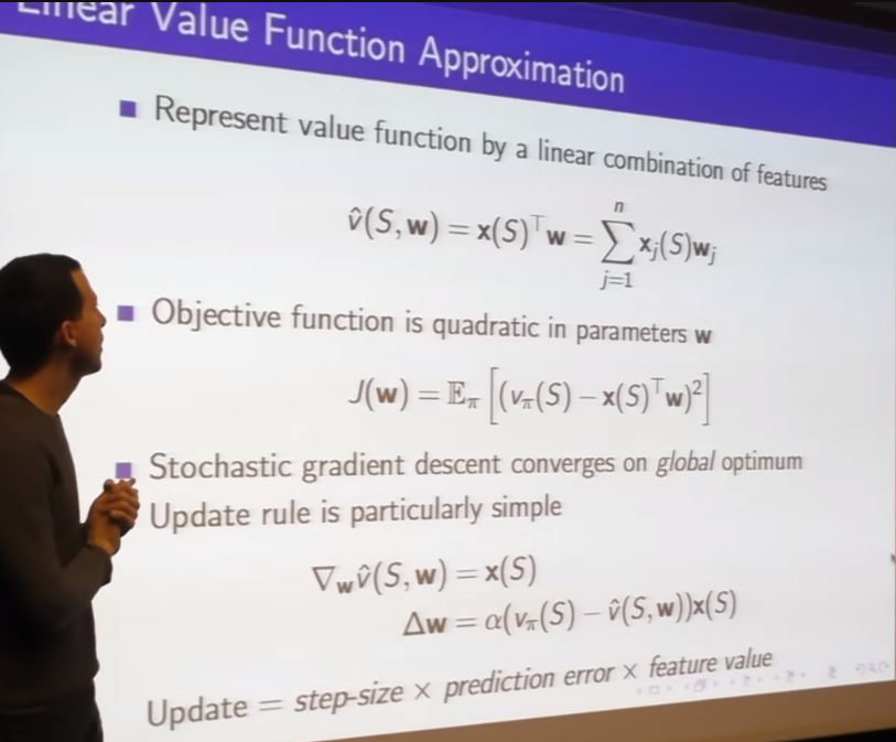
• Quadratic Equation이차방정식...

• gradident is feature vectors $x(S)$

• move your weights a little bit in the direction of the error multiplied by the feature vector

• feature vector tells you how to correct

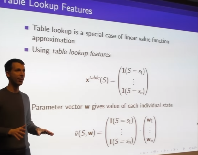
• special cases for think about

• we cheated

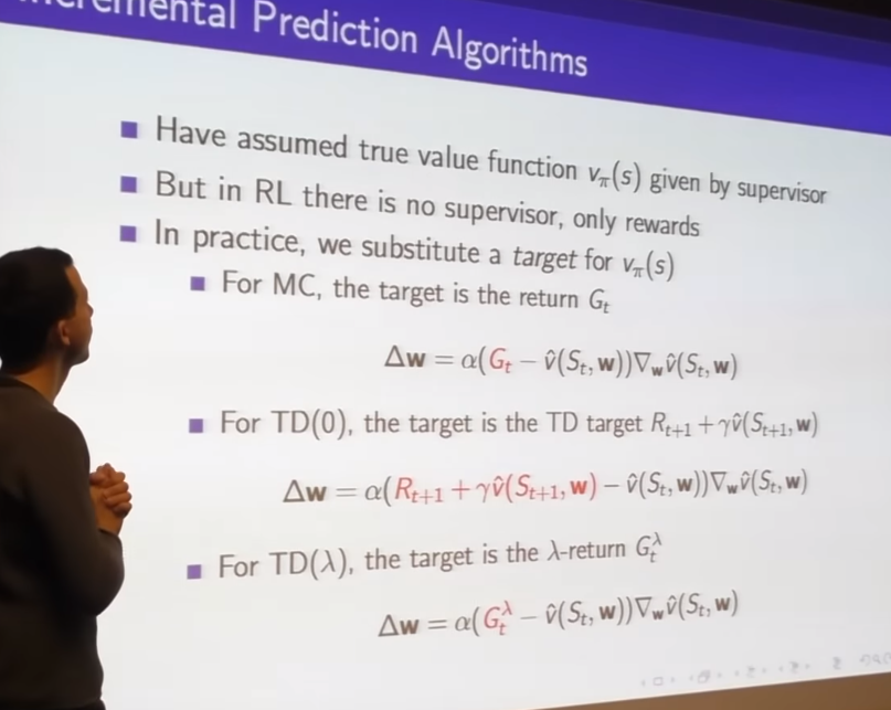
• $\Delta w$ change our weight
• we're fitting our value vunction toward the returns, kind of supervisor learning on the returns

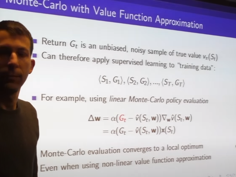
• even if we use non-linear value function approximation MC will converge to some local optimum or in the linear case it will find the global optimum

• we get

  • reward
    $R_{t+1}$
  • and query our own function approximator to estimate how much reward going to get for the rest of trajectory
    $\gamma \hat{v}(S_{t+1}, w)$

• we get
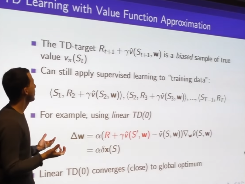
  biased sample of true alue

• TD target : one step estimate

• $\Delta w$ = $\alpha(R + \gamma \hat{v}(S^\prime, w) - \hat{v}(S,w))\nabla_w\hat{v}(S,w)$

  • step size
    $\alpha$
  • the error between what I thought the value was going to be and my one step estimate of the value
    $(R + \gamma \hat{v}(S^\prime, w) - \hat{v}(S,w))$
  • gradient tells you how to adjust your function approximator
    $\nabla_w\hat{v}(S,w)$

• $\alpha\delta x(S)$

  • stepsize x TD error x gradient(non-linear case) or feature vector(linear case)

Incremental online update

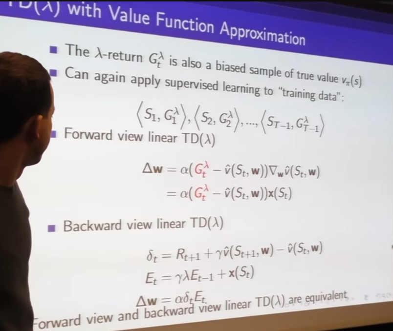
• we online update with using eligibility traces

  • eligibilities on the features(weights) of parameter vectors(size of your parameters not states)
    so eligibility accumulating credit for things that happen most and happen recently

• $\Delta w = \alpha\delta_{t}E_{t}$

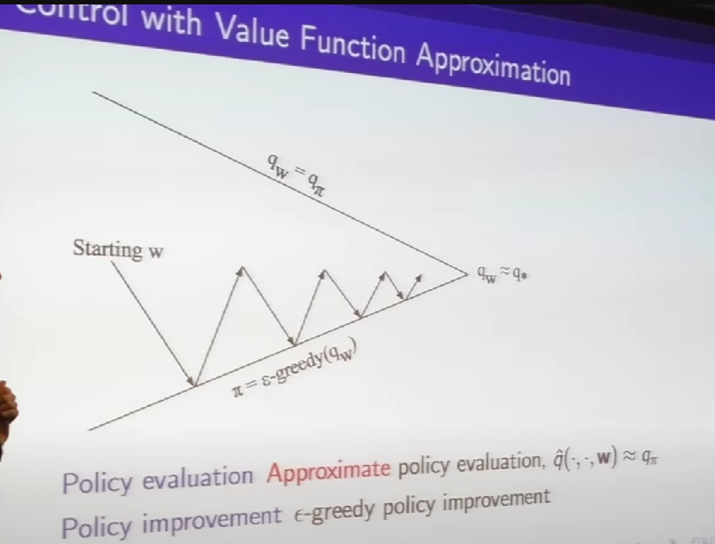
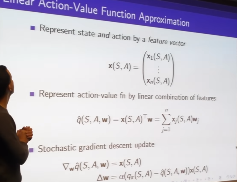
• build features of both state and action

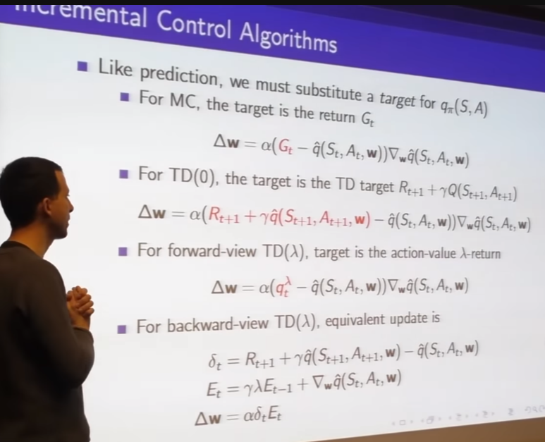
• if there is no Oracle(hypothetical perfect information source that can provide the true value or the optimal action in any given state)
  • we can use return as a noisy unbiased estimate of the Oracle
  • one-step TD target
  • lambda return
  • backward view TD lambda use eligibility traces
• difference is we using Q rather than V; so we can do control
  • once we have q we can pick the max over our actions, we don't need model
  • we can figure out what the next action we should take is and continue to do our policy improvement step

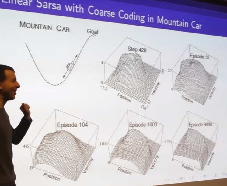
• simple function approximator is sufficient to express quite a complicated shape in value function

-eventually

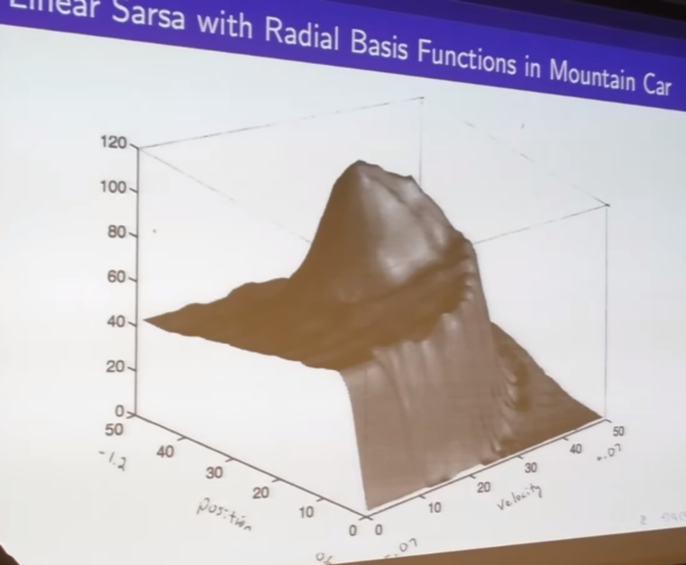
• radial based function approximator
• this is an approximation of the optimal vlue function for mounting car

continuos state space
action is discrete accelerate or not accelerate; amount of accelerate is given
-> could be continuous

• if you know good feature you can transform this complicate shape more simple one
• this is V$\pi$ but you can put knowledge in to help figure out this shape of V$\pi$ more effectively

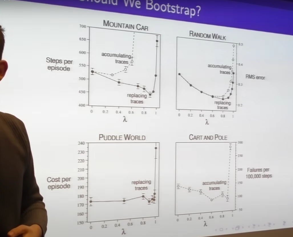
• typically TD0 is better than MC(very huge variance) and lambda is better TD0
  • we have to find sweet spot between those
  • finding algorithms effective when bootstrap

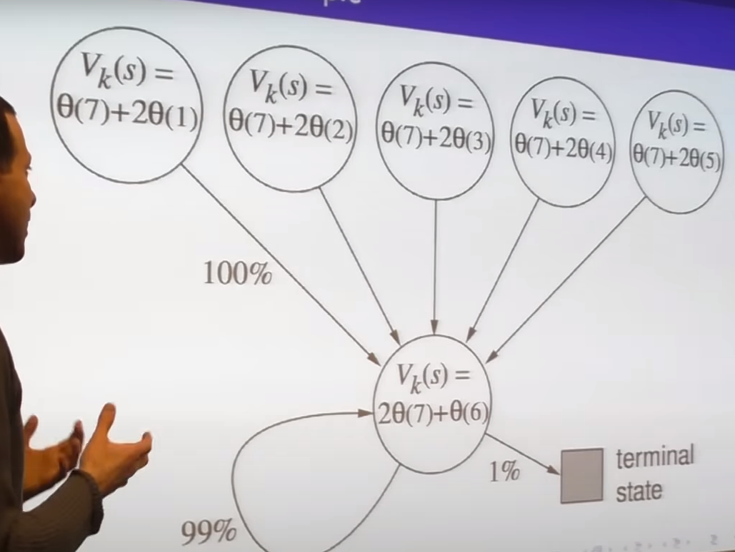
• simple MDP

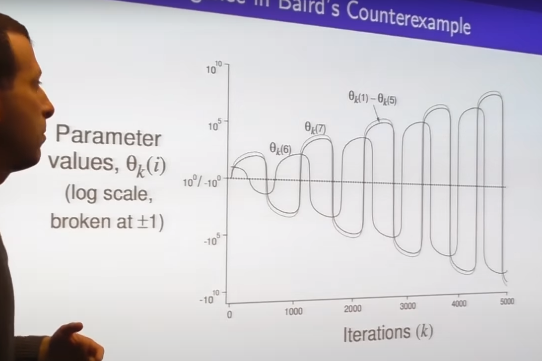
• blow up
• TD doesn't guarantee safety

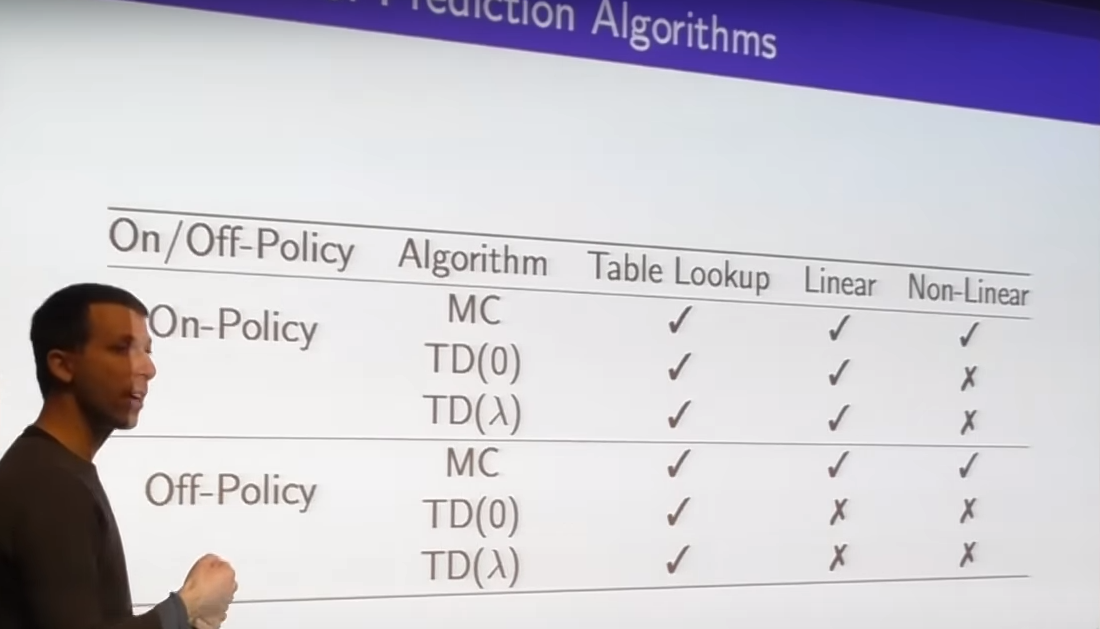
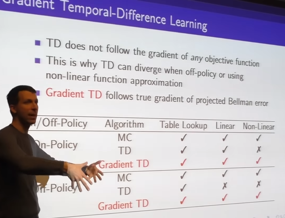
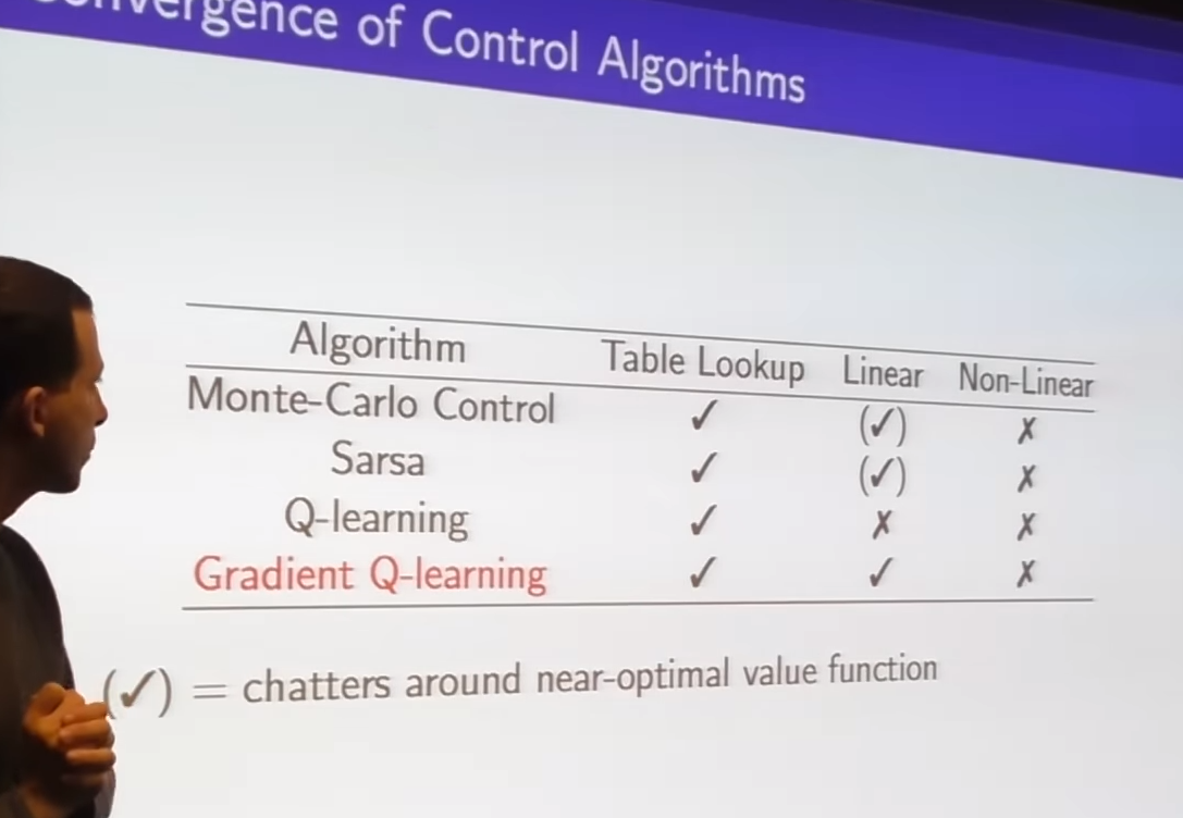
• chattering - getting closer but occasionally stepping away but never shoot off to infinity

• issue 1: is it converge to fixed point

• issue 2: if converged is it right fixed point we want

Batch Methods

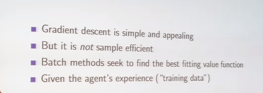
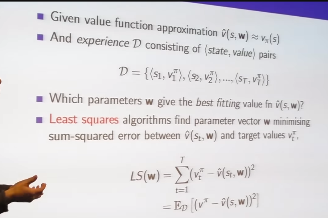
• minimize squared error between oracle value and what we thought would happen

• least square solution

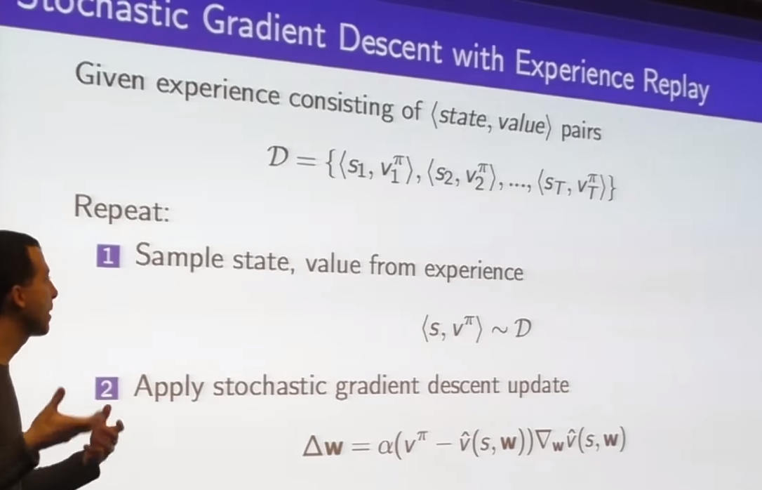
• given state s we're going to sample from experience and oracle said I should do this

• do one stochastic gradient update toward target $v^{\pi}$

  • standard supervised learning
  • made dataset, randomly sample from that data, update in the direction of our random sample

• just stochastic gradient descent update untill we get

• least square solution

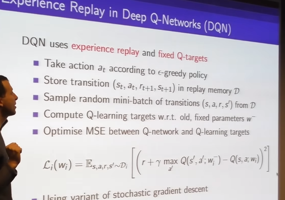
• sarsa and TD can blow up with neural networks however this method is stable with neural networks
• two tricks
  • experience replay
    • it decorrelates the trajectories
  • bootstrap towards our frozen(from some steps ago) target
    • do not bootstrap directly towards the thing which we're updating at that moment; lots of correlation between target and Q value that moment

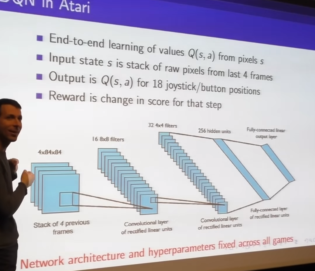
• convolutional network

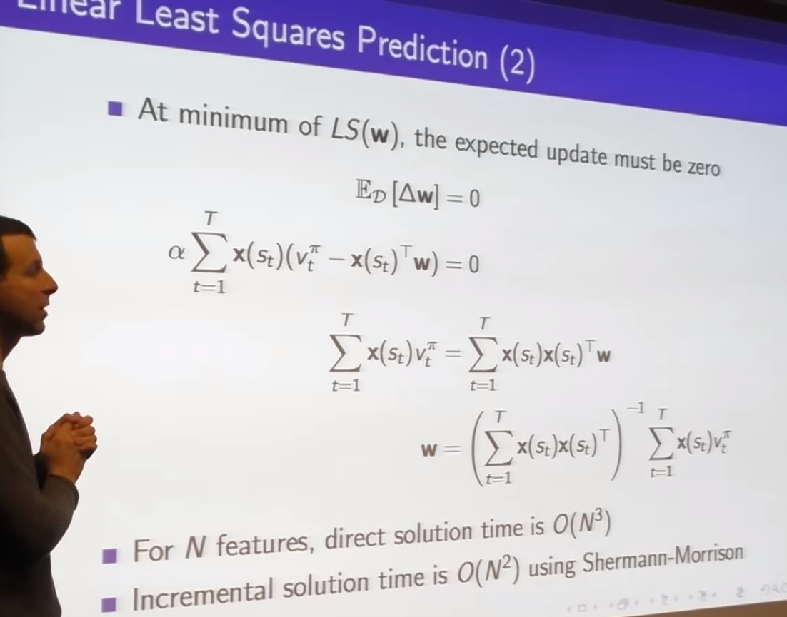
• we wouldn't make change anymore, we reached to minima

• matrix calculation cost depends on features

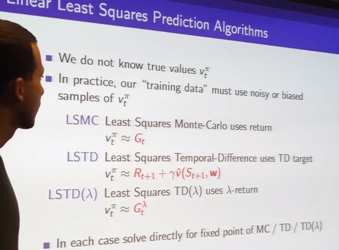
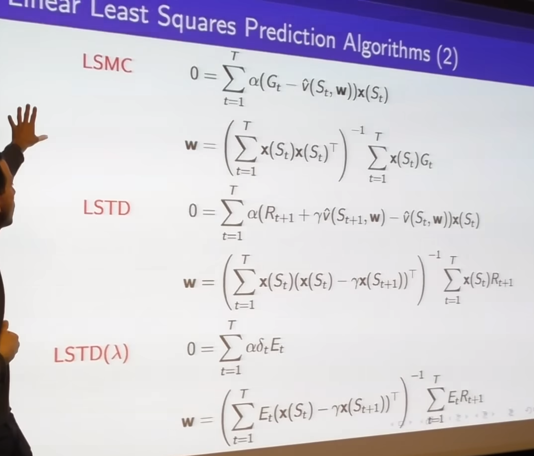
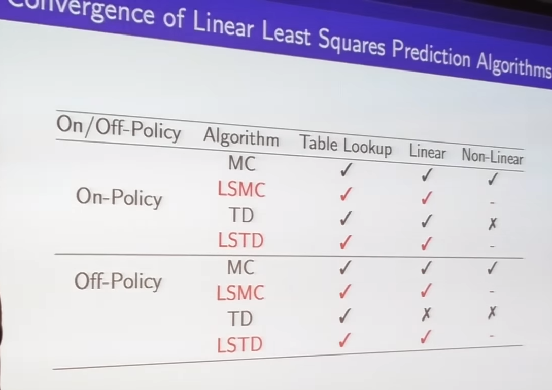
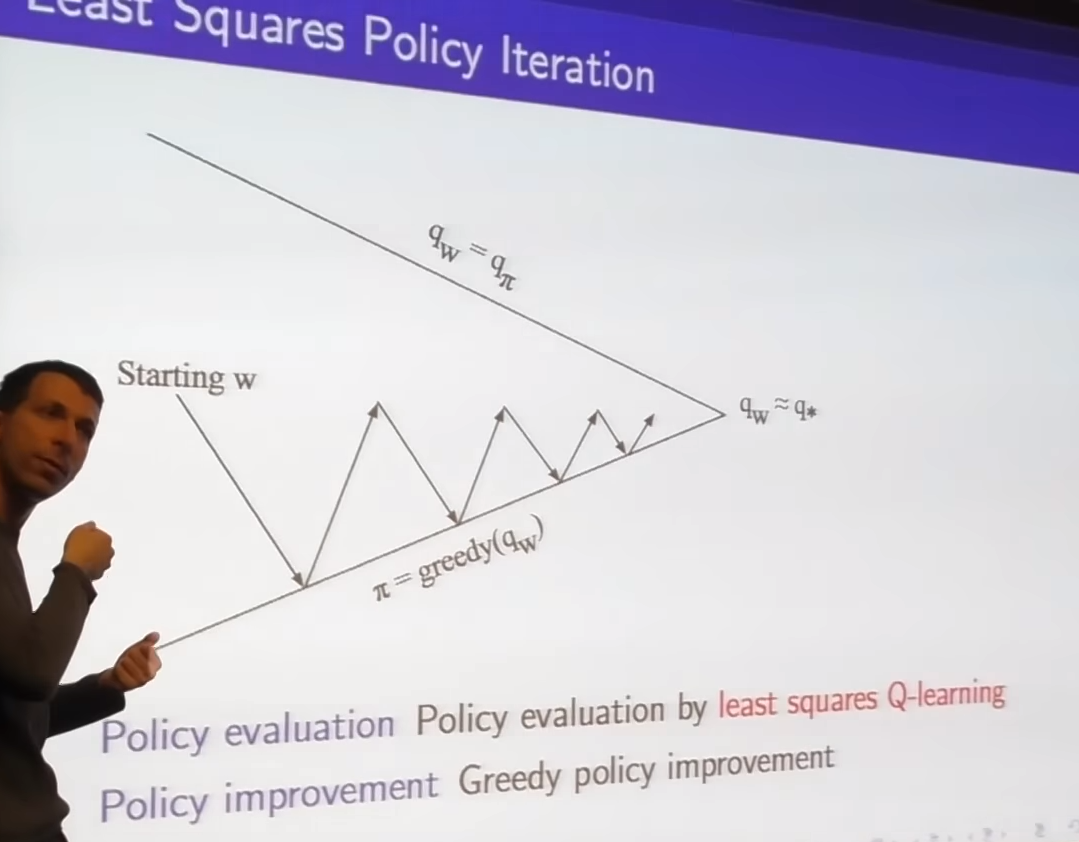
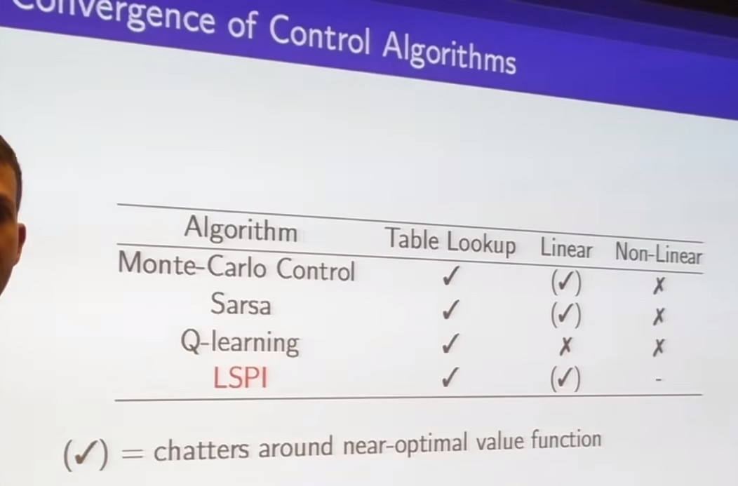
• still have issue