Duke University: Inference for a mean

Inference of a Mean

[INSTRUCTIONS]
1. Set the hypothesis

• H0: μ = suggested value
• H1: μ != suggested value

2. Check conditions
3. Calculate the point estimate x̄
4. Draw sampling distribution, calculate test statistic, shade p-value,
5. Make a decision, and interpret it in context of the research question:
   See ‘Inference_of_a_mean.pdf’ for an example

★ 2 Steps: Construct a confidence Interval → Conduct a hypothesis test

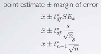
• T*df : the critical t score to be found
• Degrees of freedom for t statistic for inference on one sample mean
  • We lose one degree of freedom because we're estimating the standard error of the sample mean using the sample standard deviation.

1. Set the hypothesis

2. Check Conditions

1) Independence

• Sampled observations must be independent
  • Random sample / assignment
  • If sample without replacement, n < 10% of population

2) Sample size / skew

• The more skew in the population distributions, the higher the sample size is needed
  
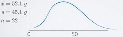
  Given the sample statistics, we can kind of sketch it out. The sample mean is 52 and there's a natural boundary at 0 since one cannot eat less than 0 grams of biscuit. So the 68, 95, 99.7 rule is just not going to apply here. Because if we go more than one standard deviation below the mean, we're going to hit that natural boundary of 0 grams. Therefore, that data are likely right skewed. The t distribution is pretty robustious units but ideally, we would like to see a visualization of this distribution and the size this sample size queue distribution accordingly, especially given the low sample size.

3. Calculate the point estimate x̄

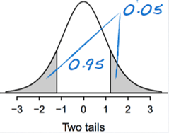
4.1 Finding the Critical T Score (table)

• Find corresponding tail area for desired confidence level
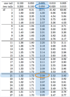
• df = 21. two tails = 0.05 → critical T score = 2.08

4.2 Construct a confidence Interval

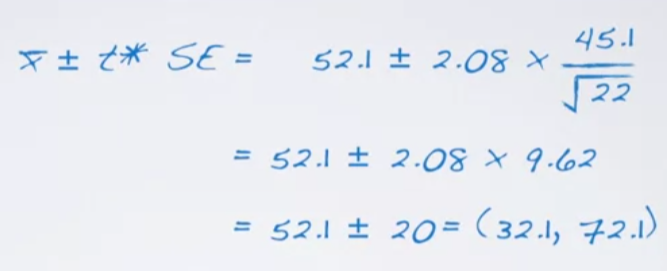
5. Make a decision, and interpret it in context of the research question

• We are 95% confident that distracted eaters consume between 32.1 to 72.1 grams of snacks post-meal.

---

※ Finding the P-value (table)

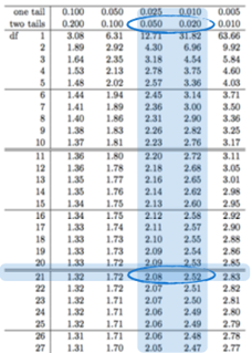
• We have df and t value. P values are on the top.
• t values are absolute so the sign is ignored.
→ 0.02 < p-value < 0.05, p-value ≒ 0.0318