Comparing Many Means(ANOVA)
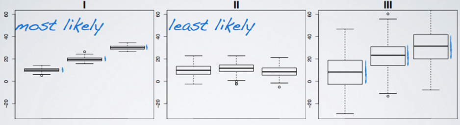
- These plots show how much groups with means are likely to be significant from each other.
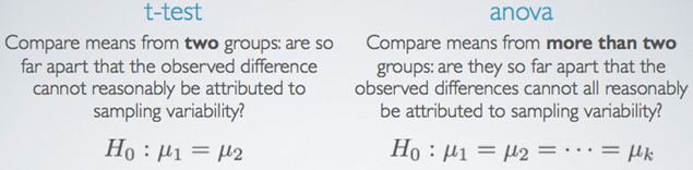
- There are more than two means to compare
- We use a new test called Analysis of Variance(ANOVA) and a new statistic called F for comparing means of 3+ groups
In ANOVA, defining the hypothesis is somewhat different from t-test
Where μi : mean of the outcome for observations in category i and k : number of groups,
H0 : The mean outcome is the same across all categories. μ1 = μ2 = … = μk
H1 : At least one pair of means are different from each other.
T – test vs ANOVA
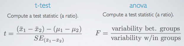
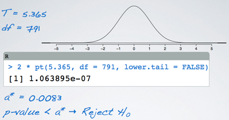
- Large test statistics lead to small p-values
- If the p-value is small enough H0 is rejected, and we conclude that the data provide evidence of a difference in the population means.
F–distribution
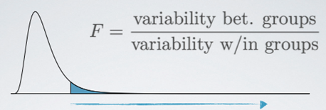
- Right skewed, always positive (since it's a ratio of two measures of variability, which can never be negative)
- In order to be able to reject H0, we need a small p-value, which requires a large F statistic
- Obtaining a large F statistic requires that the variability between sample means is greater than the variability within the samples.
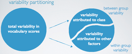
Variability Partitioning
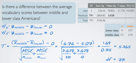
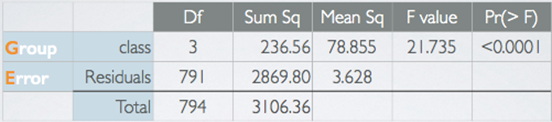
Interpreting ANOVA Output
The between-group variability is what we are interested in since it is the variability attributed to the class we are considering atm.
- ‘Group’ row: between-group variability
- ‘Error’ row: within-group variability
1) Sum of Squares Total(=SST), (Total, Sum Sq)
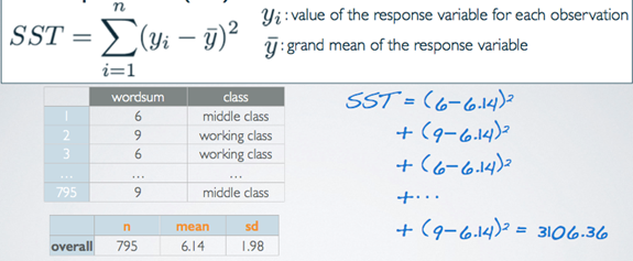
- measures the total variability in the response variable
- calculated very similarly to variance (except not scaled by the sample size)
2) Sum of Squares Groups(SSG), (Group, Sum Sq)
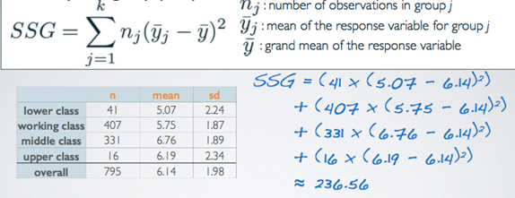
- Measures the variability between groups
- Explained variability: squared deviation of group means from overall mean, weighted by sample size
- Its own is not a meaningful number but it's interesting how it compares to the total sum of squares we calculated earlier. For example, this value is roughly 7.6% of SST. Meaning that 7.6% of the variability in vocabulary scores is explained by social class and the remainder is not explained by the explanatory variable we're considering in this analysis.
3) Sum of Squares Error(SSE), (Error, Sum Sq)
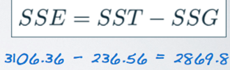
- Measures the variability within groups
- Unexplained variability: unexplained by the group variable, due to other reasons
4) Degrees of Freedom associated with ANOVA
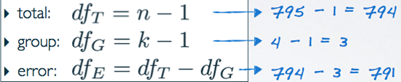
- Used to calculate the average variability from the measures of total variability(Sum Sq) as a scaling measure that incorporates sample sizes and number of groups.
5) Mean Square Error(Mean Sq)
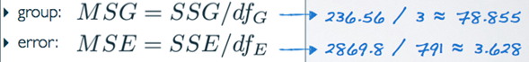
- Average variability between and within groups, calculated as the total variability (sum of squares) scaled by the associated degrees of freedom
6) F statistic
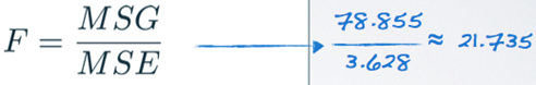
- Ratio of the average between group and within group variabilities
7) P-value
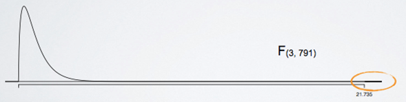
- The probability of at least as large a ratio between the “between” and “within” group variabilities if in fact the means of all groups are equal
- Area under the F curve, with degrees of freedom dfG and dfE, above the observed F statistic
ANOVA Conclusion
- If p-value is small (less than alpha), reject H0: The data provide convincing evidence that at least one pair of population means are different from each other (no tell which one though)
- If p-value is large, fail to reject H0: The data do not provide convincing evidence that at least one pair of population means are different from each other, the observed differences in sample means are attributable to sampling variability (or chance)
See ‘conditions_for_anova.pdf’
[Multiple Comparisons(사후검정)]
Which Means Differ
- Conduct two sample t tests for differences in each possible pair of groups
- And with each test that you do, you incur a probability of doing a Type I error.
- The probability of committing a Type I error is the significance level of the test, which is often set to 5%.
- So when you do multiple tests, you're going to be inflating your Type I error rate, which is an undesirable outcome.
- Thankfully, there is a simple solution.
- Use a modified significance level that is lower than the original significance level for these pairwise tests, so that the overall Type I error rate for the series of tests you have to do can still be held at the original low rate.
Multiple Comparisons
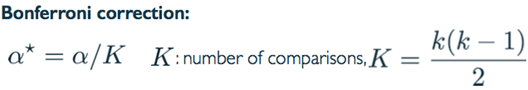
- Use Bonferroni correction for testing many pairs of groups, which suggests a more stringent significance level is more appropriate for these tests
- Adjust alpha by the number of comparisons being considered
- For example, if you have four groups in your ANOVA, and it does yield a significant result, then you need to compare group one to group two, two to three, three to four, so on and so forth. But counting these out is somewhat tedious and error prone, so we usually use a shortcut formula for determining this value and then use this value to adjust the significance level.
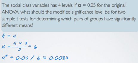
2 Steps for Bonferroni correction
1) Find the number of comparisons as k x (k - 1) / 2,
2) Correct your original alpha by this level, as alpha divided by the number of comparisons.
Example)
Other considerations when doing multiple comparisons after ANOVA
1) Constant variance
- Need to re-think standard error and degrees of freedom for all tests
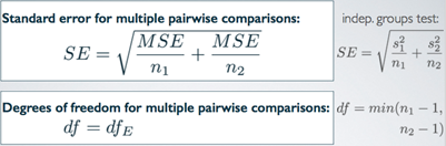
The mean's squared error is actually the average within group variance, so we're still getting at the same thing, the individual group variances, but now, we have a consistent measure that we can use for all of the tests. If, indeed, the constant variance condition is satisfied, this value should be very close to your group variances anyway.
The consistent degrees of freedom is going to be the DF error from the ANOVA output, as opposed to the minimum of the sample sizes minus one, from the two groups that we're comparing.
2) Compare the p-values from each test to the modified significance level
Example)