Iris 꽃 종류 분류
데이터는 sklearn.datasets 의 load_iris 함수를 이용해 받을 수 있습니다.

import pandas as pd
import numpy as np
import matplotlib.pyplot as plt
np.random.seed(2021)
from sklearn.datasets import load_iris
iris = load_iris()
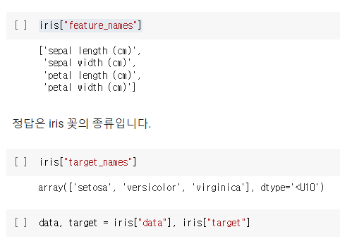
iris["feature_names"] #iris 꽃의 종류
iris["target_names"]위 코드는 파이썬에서 데이터 분석과 시각화에 자주 사용되는 패키지들인 pandas, numpy, matplotlib을 import하는 것부터 시작합니다. 그리고 난수 생성을 위해 numpy.random.seed()를 사용하여 시드값을 설정합니다.
다음으로 sklearn.datasets 패키지에서 제공하는 iris 데이터셋을 로드합니다. 이 데이터셋은 붓꽃(iris)의 꽃받침(sepal)과 꽃잎(petal)의 길이와 너비를 측정한 총 150개의 샘플이 있으며, 각 샘플은 setosa, versicolor, virginica 3가지 종류 중 하나에 속합니다.
그리고 마지막으로, iris 데이터셋에서 feature_names와 target_names를 출력하여 각각 꽃받침과 꽃잎의 길이와 너비, 그리고 꽃의 종류에 대한 레이블 정보를 확인할 수 있습니다.
데이터 EDA
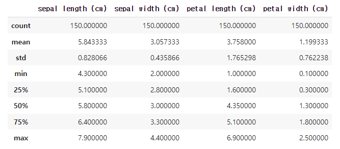
pd.DataFrame(data, columns=iris["feature_names"]).describe()위 코드는 iris 데이터셋의 feature_names를 칼럼으로 하고, data를 데이터로 갖는 pandas의 DataFrame을 생성한 뒤, describe() 메소드를 호출하여 기초 통계량을 출력합니다.
describe() 메소드는 데이터프레임의 각 열(column)에 대한 통계 정보를 요약하여 출력합니다. 이 메소드는 count(데이터 개수), mean(평균값), std(표준편차), min(최소값), 25%(1사분위수), 50%(중위값), 75%(3사분위수), max(최대값)를 출력합니다.
따라서 위 코드는 iris 데이터셋의 feature_names를 갖는 데이터프레임의 각 열에 대한 기초 통계량을 출력합니다. 이를 통해 각 열의 데이터 분포, 중심경향성, 분산정도 등을 파악할 수 있습니다.
Data Split
from sklearn.model_selection import train_test_split
train_data, test_data, train_target, test_target = train_test_split(
data, target, train_size=0.7, random_state=2021, stratify=target
)
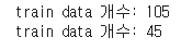
print("train data 개수:", len(train_data))
print("train data 개수:", len(test_data))위 코드는 sklearn.model_selection 패키지에서 제공하는 train_test_split() 함수를 사용하여 주어진 데이터를 train set과 test set으로 나누는 작업을 수행합니다. 이 때, train 데이터와 test 데이터를 7:3으로 나누고(train_size=0.7), 랜덤 시드값을 2021로 설정하여(random_state=2021) 매번 동일한 결과를 얻을 수 있도록 합니다. 그리고 stratify 매개변수를 이용하여 train과 test 데이터에 각각 클래스 비율이 고르게 포함되도록 데이터를 나누어 줍니다.
train_test_split() 함수는 데이터셋을 무작위로 섞은 뒤 지정한 비율에 따라 train set과 test set으로 분할합니다. 이 때, 데이터를 분할하는데에는 임의성(randomness)이 존재하므로, 매번 동일한 결과를 얻기 위해 랜덤 시드값을 지정해주는 것이 좋습니다.
마지막으로, train set과 test set의 크기를 출력하여 확인합니다. 이를 통해 train set과 test set이 각각 얼마나 많은 데이터를 가지고 있는지 확인할 수 있습니다.
시각화
fig, axes = plt.subplots(nrows=2, ncols=3, figsize=(15,10))
pair_combs = [
[0, 1], [0, 2], [0, 3], [1, 2], [1, 3], [2, 3]
]
for idx, pair in enumerate(pair_combs):
x, y = pair
ax = axes[idx//3, idx%3]
ax.scatter(
x=train_data[:, x], y=train_data[:, y], c=train_target, edgecolor='black', s=15
)
ax.set_xlabel(iris["feature_names"][x])
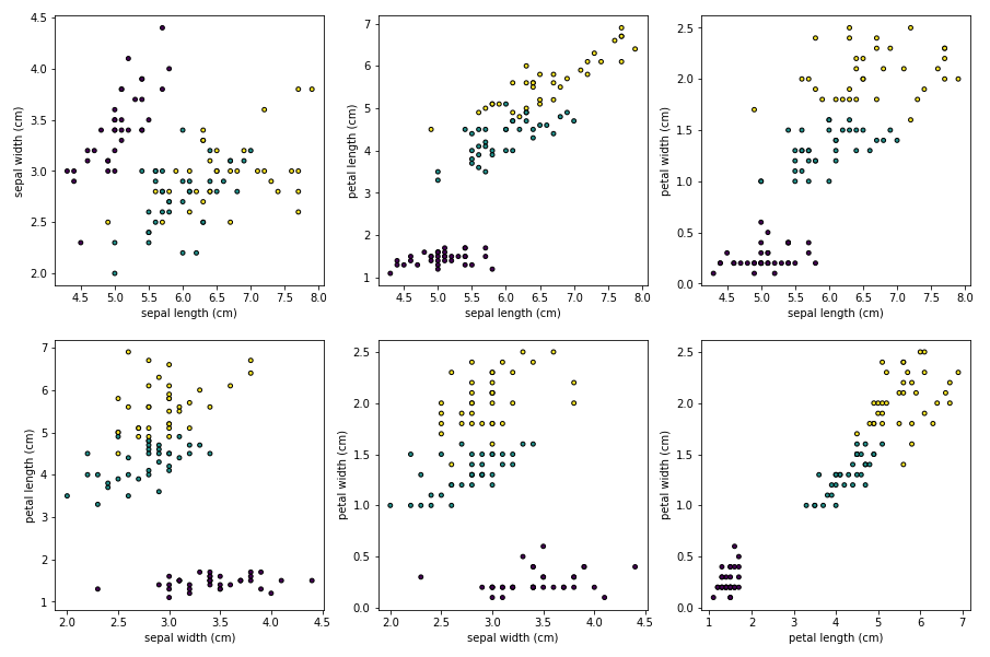
ax.set_ylabel(iris["feature_names"][y])위 코드는 matplotlib 패키지를 이용하여 scatter plot을 그리는 작업을 수행합니다.
먼저, subplots() 함수를 호출하여 2행 3열의 플롯을 생성합니다. figsize 매개변수는 그림의 크기를 지정합니다.
그리고 pair_combs라는 변수에 모든 feature 조합을 리스트로 저장합니다. 즉, 꽃받침과 꽃잎의 길이와 너비 4가지 feature를 모두 조합하여 나올 수 있는 모든 경우의 수를 저장합니다. 이 때, 한 번에 그릴 수 있는 scatter plot은 최대 6개까지이므로, 6개의 조합만을 사용합니다.
그리고 for 루프를 통해 pair_combs에 저장된 모든 조합에 대해 scatter plot을 그립니다. x, y는 각 feature의 인덱스를 나타냅니다. ax.scatter() 함수를 호출하여 scatter plot을 그립니다. 이 때, train_data의 x열과 y열 값을 사용하고, c 매개변수에는 train_target을 사용하여 클래스별로 다른 색상으로 구분되도록 합니다. edgecolor 매개변수를 사용하여 점의 테두리 색상을 지정하고, s 매개변수를 사용하여 점의 크기를 지정합니다.
마지막으로, 각 plot에 대한 x축과 y축의 라벨을 설정합니다. 이를 통해 각 plot이 어떤 feature의 조합인지 파악할 수 있습니다.
Decision Tree
from sklearn.tree import DecisionTreeClassifier, plot_tree
gini_tree = DecisionTreeClassifier()

gini_tree.fit(train_data, train_target) #학습
plt.figure(figsize=(10,10))
plot_tree(gini_tree, feature_names=iris["feature_names"], class_names=iris["target_names"])
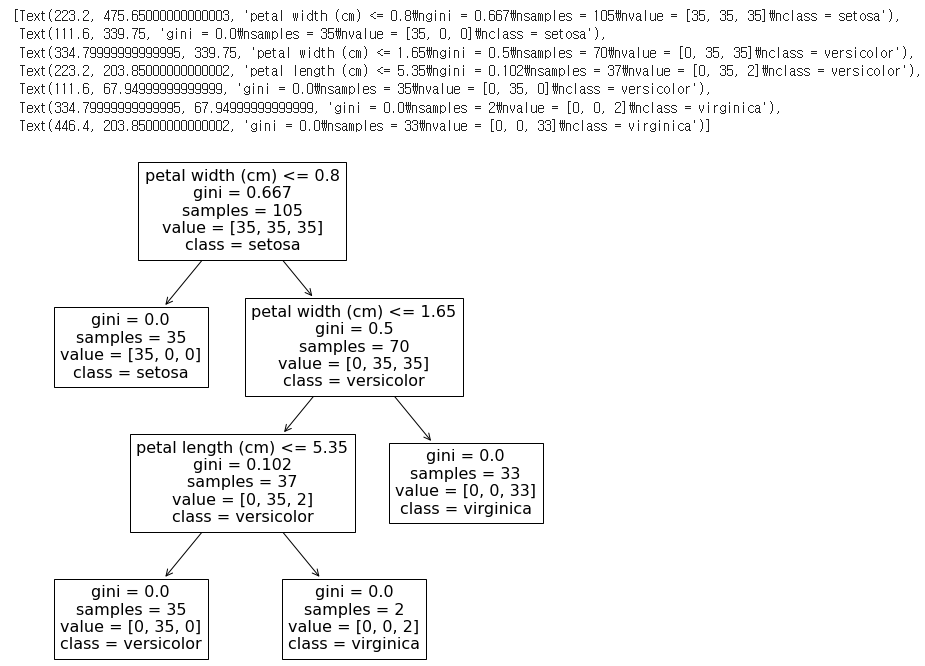
위 코드는 sklearn.tree 패키지에서 제공하는 DecisionTreeClassifier() 클래스를 이용하여 의사결정나무 모델을 학습하고, 학습된 모델을 시각화하는 작업을 수행합니다.
먼저, DecisionTreeClassifier() 클래스를 호출하여 gini_tree라는 이름의 객체를 생성합니다.
그리고 gini_tree.fit() 함수를 사용하여 train_data와 train_target 데이터를 이용하여 의사결정나무 모델을 학습합니다.
마지막으로, plot_tree() 함수를 호출하여 학습된 모델을 시각화합니다. feature_names 매개변수에는 iris 데이터셋의 feature_names 정보를 전달하고, class_names 매개변수에는 iris 데이터셋의 target_names 정보를 전달합니다. 이를 통해 의사결정나무의 각 노드에서 사용된 feature 이름과 클래스 이름을 확인할 수 있습니다. figsize 매개변수를 사용하여 그림의 크기를 조정할 수 있습니다.
Arguments
DecisionTreeClassifier에서 주로 탐색하는 argument들은 다음과 같습니다.
- criterion
어떤 정보 이득을 기준으로 데이터를 나눌지 정합니다.
"gini", "entropy" - max_depth
나무의 최대 깊이를 정해줍니다. - min_samples_split
노드가 나눠질 수 있는 최소 데이터 개수를 정합니다.
1) max_depth
depth_1_tree = DecisionTreeClassifier(max_depth=1)
depth_1_tree.fit(train_data, train_target)
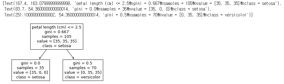
plot_tree(depth_1_tree, feature_names=iris["feature_names"], class_names=iris["target_names"])위 코드는 max_depth 매개변수를 이용하여 의사결정나무의 최대 깊이를 설정하고, 학습된 모델을 시각화하는 작업을 수행합니다.
먼저, DecisionTreeClassifier() 클래스를 호출하고, max_depth 매개변수에 1을 전달하여 depth_1_tree라는 이름의 객체를 생성합니다. 이를 통해 의사결정나무의 최대 깊이를 1로 제한합니다.
그리고 depth_1_tree.fit() 함수를 사용하여 train_data와 train_target 데이터를 이용하여 의사결정나무 모델을 학습합니다.
마지막으로, plot_tree() 함수를 호출하여 학습된 모델을 시각화합니다. feature_names 매개변수에는 iris 데이터셋의 feature_names 정보를 전달하고, class_names 매개변수에는 iris 데이터셋의 target_names 정보를 전달합니다. 이를 통해 의사결정나무의 각 노드에서 사용된 feature 이름과 클래스 이름을 확인할 수 있습니다.
2) min_samples_split
sample_50_tree = DecisionTreeClassifier(min_samples_split=50)
sample_50_tree.fit(train_data, train_target)
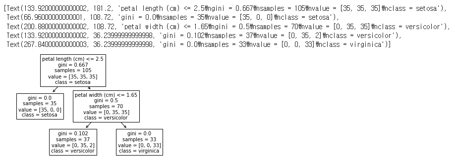
plot_tree(sample_50_tree, feature_names=iris["feature_names"], class_names=iris["target_names"])위 코드는 min_samples_split 매개변수를 이용하여 노드를 분할하기 위한 최소 샘플 수를 설정하고, 학습된 모델을 시각화하는 작업을 수행합니다.
먼저, DecisionTreeClassifier() 클래스를 호출하고, min_samples_split 매개변수에 50을 전달하여 sample_50_tree라는 이름의 객체를 생성합니다. 이를 통해 노드를 분할하기 위한 최소 샘플 수를 50으로 제한합니다.
그리고 sample_50_tree.fit() 함수를 사용하여 train_data와 train_target 데이터를 이용하여 의사결정나무 모델을 학습합니다.
마지막으로, plot_tree() 함수를 호출하여 학습된 모델을 시각화합니다. feature_names 매개변수에는 iris 데이터셋의 feature_names 정보를 전달하고, class_names 매개변수에는 iris 데이터셋의 target_names 정보를 전달합니다. 이를 통해 의사결정나무의 각 노드에서 사용된 feature 이름과 클래스 이름을 확인할 수 있습니다.
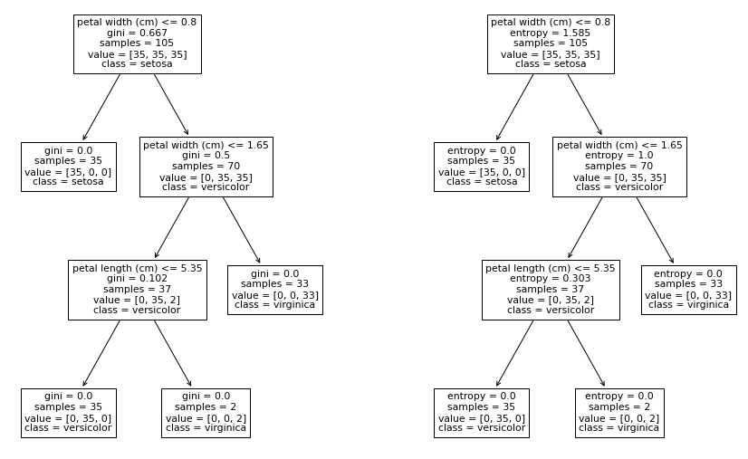
3) criterion
entropy_tree = DecisionTreeClassifier(criterion="entropy")
entropy_tree.fit(train_data, train_target)

fig, axes = plt.subplots(nrows=1, ncols=2, figsize=(15, 10))
plot_tree(gini_tree, feature_names=iris["feature_names"], class_names=iris["target_names"], ax=axes[0])
plot_tree(entropy_tree, feature_names=iris["feature_names"], class_names=iris["target_names"], ax=axes[1])
plt.show()
위 코드는 criterion 매개변수를 이용하여 의사결정나무 모델에서 사용할 분리 기준을 entropy로 설정하고, 이를 시각화하는 작업을 수행합니다.
먼저, DecisionTreeClassifier() 클래스를 호출하고, criterion 매개변수에 "entropy"를 전달하여 entropy_tree라는 이름의 객체를 생성합니다. 이를 통해 의사결정나무 모델에서 사용할 분리 기준을 entropy로 설정합니다.
그리고 entropy_tree.fit() 함수를 사용하여 train_data와 train_target 데이터를 이용하여 의사결정나무 모델을 학습합니다.
마지막으로, subplots() 함수를 사용하여 2개의 subplot을 가지는 figure 객체를 생성합니다. 그리고 plot_tree() 함수를 호출하여 각각의 subplot에 gini_tree와 entropy_tree를 시각화합니다. feature_names 매개변수에는 iris 데이터셋의 feature_names 정보를 전달하고, class_names 매개변수에는 iris 데이터셋의 target_names 정보를 전달합니다. 이를 통해 의사결정나무의 각 노드에서 사용된 feature 이름과 클래스 이름을 확인할 수 있습니다.
예측
trees = [
("gini tree", gini_tree),
("entropy tree", entropy_tree),
("depth=1 tree", depth_1_tree),
("sample=50 tree" ,sample_50_tree),
]
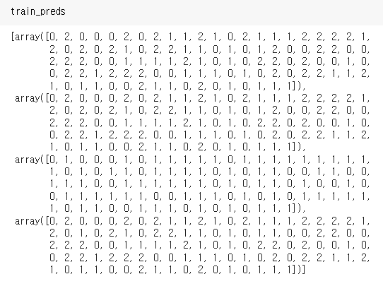
train_preds = []
test_preds = []
for tree_name, tree in trees:
train_pred = tree.predict(train_data)
test_pred = tree.predict(test_data)
train_preds += [train_pred]
test_preds += [test_pred]위 코드는 앞서 생성한 4개의 의사결정나무 모델을 이용하여 train_data와 test_data를 예측하는 작업을 수행합니다.
먼저, 의사결정나무 모델을 리스트 형태로 저장합니다. 이 때, 각 모델의 이름과 해당 모델 객체를 저장합니다.
그리고 for loop을 사용하여, 각 모델을 이용하여 train_data와 test_data를 예측합니다. 예측 결과를 각각 train_pred와 test_pred에 저장합니다. 이를 위해 각각의 리스트(train_preds, test_preds)에 train_pred와 test_pred를 추가합니다.
이를 통해, 각 모델의 예측 결과를 train_preds와 test_preds에 저장하게 됩니다.
평가하기
from sklearn.metrics import accuracy_score
for idx, (tree_name, tree) in enumerate(trees):
    train_acc = accuracy_score(train_target, train_preds[idx])
    test_acc =  accuracy_score(test_target, test_preds[idx])
    print(tree_name)
    print("\t", f"train accuracy is {train_acc:.2f}")
    print("\t", f"test accuracy is {test_acc:.2f}")
위 코드는 앞서 생성한 4개의 의사결정나무 모델을 이용하여 train_data와 test_data를 예측한 결과를 이용하여 각 모델의 정확도를 평가하는 작업을 수행합니다.
for loop을 사용하여, 각 모델의 이름과 해당 모델 객체를 순회하면서, 각 모델의 train_data와 test_data에 대한 예측 결과(train_preds[idx], test_preds[idx])를 이용하여 정확도를 계산합니다.
이를 위해, accuracy_score 함수를 사용합니다. 이 함수는 정답 데이터와 예측 결과 데이터를 입력으로 받아 정확도를 계산합니다. 계산된 train 데이터와 test 데이터의 정확도를 출력합니다.
Feature Importance
iris["feature_names"] #iris 데이터셋의 feature names를 출력
gini_tree.feature_importances_ #gini_tree 모델에서 feature importance를 추출하여, 이를 Series 형태로 변환, Series의 index는 iris 데이터셋의 feature names로 설정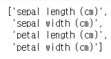
gini_feature_importance = pd.Series(gini_tree.feature_importances_, index=iris["feature_names"])
#gini_tree 모델의 feature importance를 시각화합니다. plot 함수의 인자로 kind="barh"를 전달하여 수평 막대 그래프로 시각화하고, title을 설정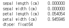
gini_feature_importance.plot(kind="barh", title="gini tree feature importance")
# sample_50_tree 모델에서 feature importance를 추출하여, 이를 Series 형태로 변환합니다. Series의 index는 iris 데이터셋의 feature names로 설정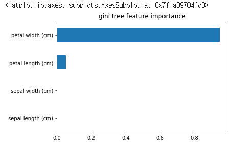
sample_50_feature_importance = pd.Series(
    sample_50_tree.feature_importances_,
    index=iris["feature_names"]
)

sample_50_feature_importance.plot(kind="barh", title="sample=50 tree feature importance")

# sample_50_tree 모델의 feature importance를 시각화합니다. plot 함수의 인자로 kind="barh"를 전달하여 수평 막대 그래프로 시각화하고, title을 설정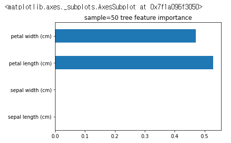
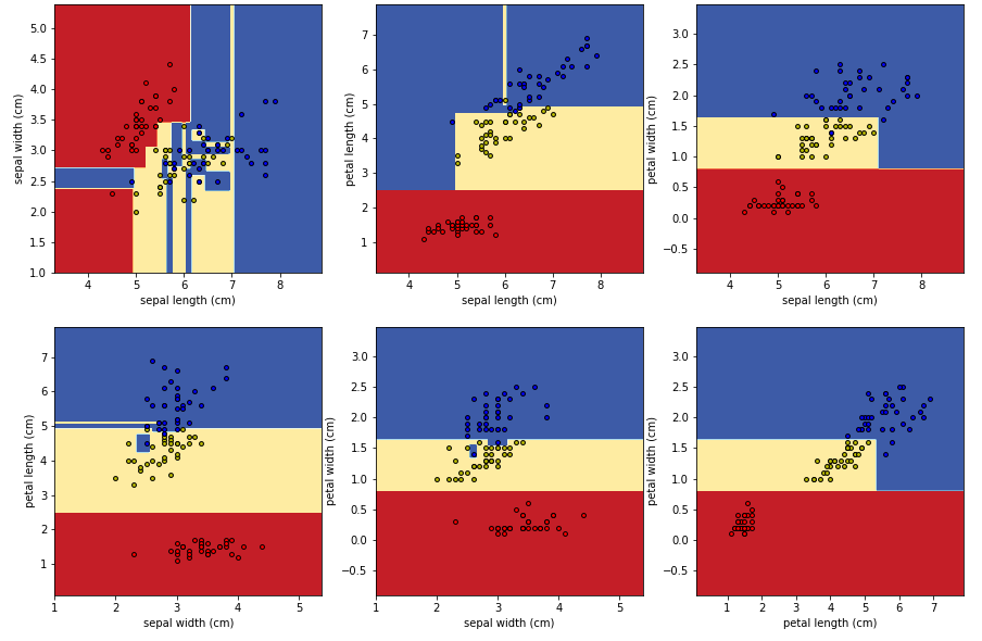
시각화
def plot_decision_boundary(pair_data, pair_tree, ax):
    x_min, x_max = pair_data[:, 0].min() - 1, pair_data[:, 0].max() + 1
    y_min, y_max = pair_data[:, 1].min() - 1, pair_data[:, 1].max() + 1
    xx, yy = np.meshgrid(np.arange(x_min, x_max, 0.02),
                         np.arange(y_min, y_max, 0.02))

    Z = pair_tree.predict(np.c_[xx.ravel(), yy.ravel()])
    Z = Z.reshape(xx.shape)
    cs = ax.contourf(xx, yy, Z, cmap=plt.cm.RdYlBu)

    # Plot the training points
    for i, color in zip(range(3), "ryb"):
        idx = np.where(train_target == i)
        ax.scatter(pair_data[idx, 0], pair_data[idx, 1], c=color, label=iris["target_names"][i],
                    cmap=plt.cm.RdYlBu, edgecolor='black', s=15)
    return ax

    fig, axes = plt.subplots(nrows=2, ncols=3, figsize=(15,10))

fig, axes = plt.subplots(nrows=2, ncols=3, figsize=(15,10))

pair_combs = [    [0, 1], [0, 2], [0, 3], [1, 2], [1, 3], [2, 3]
]
for idx, pair in enumerate(pair_combs):
    x, y = pair
    pair_data = train_data[:, pair]
    pair_tree = DecisionTreeClassifier().fit(pair_data, train_target)

    ax = axes[idx//3, idx%3]
    plot_decision_boundary(pair_data, pair_tree, ax)
    ax.set_xlabel(iris["feature_names"][x])
    ax.set_ylabel(iris["feature_names"][y])
위 코드는 서브플롯 그리드를 생성하고 각 특징 쌍에 대한 결정 경계를 각 서브플롯에 그리도록합니다.