스팸 문자를 Naive Bayes를 이용해 분류하기
sms_spam.csv 데이터는 문자 내용이 스팸인지 아닌지를 구분하기 위한 데이터이다
현재 작업 중인 디렉토리에 "sms_spam.csv" 파일이 있어야 아래 코드가 실행된다!
import pandas as pd
import numpy as np
import matplotlib.pyplot as plt

np.random.seed(2021)

#"sms_spam.csv" 파일을 pandas의 read_csv() 함수를 이용하여 읽어와 spam이라는 변수에 저장
spam = pd.read_csv("sms_spam.csv")

#spam 변수에서 "text" 열과 "type" 열을 각각 text와 label 변수에 저장
text = spam["text"]
label = spam["type"]
Data EDA
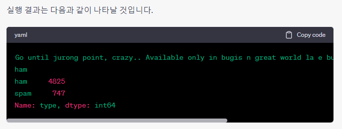
# 첫 번째 메시지 내용 출력
print(text[0])
# 첫 번째 메시지 분류 결과 출력
print(label[0])
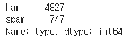
# 분류 결과별 빈도수 출력
print(label.value_counts())
Data Cleaning
정답의 문자를 숫자로 변환시켜줍니다.
ham은 0으로, spam은 1로 변환 시켜주겠습니다.
label = label.map({"ham": 0, "spam": 1}) #시리즈 객체 내의 값 중 "ham"은 0으로, "spam"은 1로 매핑하여 새로운 시리즈 객체를 생성
label.value_counts() #업데이트된 label 시리즈 객체 내에 있는 값들의 빈도수를 세어 반환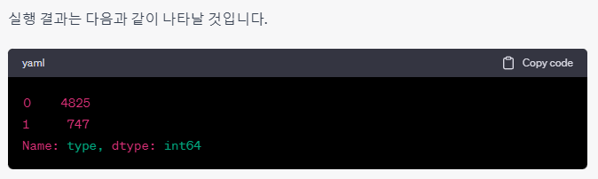
text를 문자만 존재하도록 정리해줍니다.
regex를 통해 영어, 숫자 그리고 띄어쓰기를 제외한 모든 단어를 지우도록 하겠습니다.
re_pattern = "[^a-zA-Z0-9\ ]"
text[0]
text.iloc[:1].str.replace(re_pattern, "", regex=True)[0]
text = text.str.replace(re_pattern, "", regex=True)
위 코드는 정규표현식(re_pattern)을 사용하여 text 데이터에서 영문자, 숫자, 공백을 제외한 모든 문자를 제거하는 과정입니다.
먼저 text 데이터에서 0번째 값을 확인해보면 "Go until jurong point, crazy.. Available only in bugis n great world la e buffet... Cine there got amore wat..." 와 같은 형태로 특수문자, 대소문자가 혼용된 문자열 데이터입니다.
이후 re_pattern을 적용하여 text 데이터에서 정규표현식에 해당하는 문자열을 제거하고, 공백으로 대체하는 과정을 거쳐 정제된 문자열 데이터를 저장합니다. 최종적으로 text 변수에 정제된 문자열 데이터가 저장됩니다.
그리고 나서 대문자들을 모두 소문자로 바꿔 줍니다.
text[0] # Go until jurong point, crazy.. Available only in bugis n great world la e buffet... Cine there got amore wat...

text.iloc[:1].str.lower()[0] # go until jurong point, crazy.. available only in bugis n great world la e buffet... cine there got amore wat...

text = text.str.lower() # 모든 문장을 소문자로 변경

text[0] # go until jurong point, crazy.. available only in bugis n great world la e buffet... cine there got amore wat...
Data Split
from sklearn.model_selection import train_test_split

train_text, test_text, train_label, test_label = train_test_split(
    text, label, train_size=0.7, random_state=2021
)
print(f"train_data size: {len(train_label)}, {len(train_label)/len(text):.2f}")
print(f"test_data size: {len(test_label)}, {len(test_label)/len(text):.2f}")
train_test_split 함수를 이용해 전체 데이터(text)를 70%의 학습 데이터(train_text, train_label)와 30%의 테스트 데이터(test_text, test_label)로 분할하고, 각각의 데이터 크기와 전체 데이터 대비 비율을 출력하고 있다.
train_size=0.7은 학습 데이터의 비율을 70%로 설정하며, random_state는 분할 시 샘플링 방식을 일관성 있게 유지하기 위해 설정한 시드 값이다.
따라서 실행 결과로는 학습 데이터 크기와 비율, 테스트 데이터 크기와 비율이 출력될 것이다.
Count Vectorize
이제 Naive Bayes를 학습시키기 위해서 각 문장에서 단어들이 몇 번 나왔는지로 변환해야 합니다.
- word tokenize
문장을 단어로 나누는 데에는 nltk 패키지의 word_tokenize를 이용합니다.
#NLTK 패키지를 사용하여 train 데이터셋의 첫번째 텍스트 문장을 토큰화(Tokenize)하는 과정
import nltk
from nltk import word_tokenize

nltk.download('punkt')

train_text.iloc[0]
word_tokenize(train_text.iloc[0])

pd.DataFrame(sample_cnt_vector, columns=vocab)
NLTK 패키지에서는 word_tokenize 함수를 이용하여 문장을 단어 단위로 쪼개주는 기능을 제공한다.
위 코드에서는 먼저 nltk 패키지를 import 하고, punkt 데이터를 다운로드 받습니다.
이후 train_text 데이터셋의 첫번째 문장을 word_tokenize 함수를 이용하여 단어 단위로 쪼개줍니다.
해당 코드의 실행 결과는 첫번째 train_text 문장이 단어 단위로 분리된 리스트 형태로 출력됩니다.
count vectorize
다음은 sklearn.feature_extraction.text의 CountVectorizer를 이용해 단어들을 count vector로 만들어 보겠습니다.
- 우선 예시로 2개의 문장으로 CountVectorizer를 학습
아래는 train 데이터의 첫 번째와 두 번째 텍스트를 가지고 단어 빈도수 벡터화를 수행하는 코드
train_text.iloc[:2].values #train 데이터의 첫 번째와 두 번째 텍스트를 얻음
cnt_vectorizer.fit(train_text.iloc[:2]) #각 단어의 빈도수를 세는 CountVectorizer 모델을 학습, 이때 fit 메소드는 주어진 텍스트 데이터를 이용해 단어 사전(vocabulary)을 만드는 역할

cnt_vectorizer.vocabulary_ #CountVectorizer 모델에서 만들어진 단어 사전의 각 단어가 어떤 인덱스에 매핑되었는지를 확인가능

vocab = sorted(cnt_vectorizer.vocabulary_.items(), key=lambda x: x[1])
vocab = list(map(lambda x: x[0], vocab))
vocab

sample_cnt_vector = cnt_vectorizer.transform(train_text.iloc[:2]).toarray()
sample_cnt_vector

train_text.iloc[:2].values
vocab = sorted(cntvectorizer.vocabulary.items(), key=lambda x: x[1])는 단어 사전을 (단어, 인덱스)의 쌍으로 구성된 튜플 리스트로 변환하고, 이를 인덱스를 기준으로 오름차순으로 정렬한 후, 단어만 추출하여 리스트로 저장합니다.
sample_cnt_vector = cnt_vectorizer.transform(train_text.iloc[:2]).toarray()는 CountVectorizer 모델을 이용해 train 데이터의 첫 번째와 두 번째 텍스트에서 각 단어의 빈도수를 카운트하여 희소 행렬(sparse matrix) 형태로 표현한 후, 이를 dense matrix로 변환하여 저장합니다.
마지막으로 train_text.iloc[:2].values를 출력하여 첫 번째와 두 번째 텍스트가 벡터화 되어있는 것을 확인할 수 있습니다.
- 이제 모든 데이터에 대해서 학습을 진행하겠습니다.
cnt_vectorizer = CountVectorizer(tokenizer=word_tokenize)
cnt_vectorizer.fit(train_text)

len(cnt_vectorizer.vocabulary_) #전체 단어는 7908개가 존재- 예측
train_matrix = cnt_vectorizer.transform(train_text)
test_matrix = cnt_vectorizer.transform(test_text)
만약 존재하지 않는 단어가 들어올 경우 어떻게 될까요?
CountVectorize는 학습한 단어장에 존재하지 않는 단어가 들어오게 될 경우 무시합니다.
cnt_vectorizer.transform(["notavailblewordforcnt"]).toarray().sum() #0출력위 코드는 훈련 데이터와 테스트 데이터를 각각 단어 출현 빈도수를 통해 변환해주는 코드입니다. 훈련 데이터에는 train_text와 train_label이 있으며, 테스트 데이터에는 test_text와 test_label이 있습니다. 각각의 데이터는 CountVectorizer를 통해 단어 출현 빈도수를 계산한 후에 transform 메서드를 통해 변환됩니다. 이를 통해 각 문장에서 단어들이 몇 번씩 나왔는지를 벡터 형태로 표현하여 분석에 활용할 수 있게 됩니다.
Naive Bayes
분류를 위한 Naive Bayes 모델은 sklearn.naive_bayes의 BernoulliNB를 사용
from sklearn.naive_bayes import BernoulliNB
naive_bayes = BernoulliNB()

#학습
naive_bayes.fit(train_matrix, train_label)

#예측
train_pred = naive_bayes.predict(train_matrix)
test_pred = naive_bayes.predict(test_matrix)

#평가
from sklearn.metrics import accuracy_score

train_acc = accuracy_score(train_label, train_pred)
test_acc = accuracy_score(test_label, test_pred)

print(f"Train Accuracy is {train_acc:.4f}")
print(f"Test Accuracy is {test_acc:.4f}")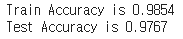
학습 데이터에 대한 정확도는 0.9926이고, 테스트 데이터에 대한 정확도는 0.9849입니다.