17. Metric Learning
-
Task
- Metric learning is the task of learning a distance function over objects.
- A model takes two or more examples and outputs a (non-negative) score.
- The distance may have different meaning depending on the data.
- The model will learn the relationship in the training data, whatever it actually means.
-
Data
- (weakly) Supervised learning
- But, often with free of human labor
- Relative similarity data is easier to collect than traditional labeled one.
- Photos taken at the same place
- Videos watched in the same YouTube session
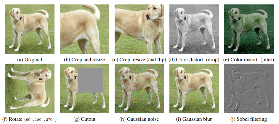
- Data augmentation
- Ordinal regression
- Map to an ordered set of classes
- (weakly) Supervised learning
17.1. Learning to Rank
Training data consists of lists of items with some partial order specified between items in each list. The ranking model purposes to rank, i.e., producing a permutation of items in new, unseen lists in a similar way to rankings in the training data.
-
Problem Formulation
- Point-wise
- Pair-wise
- Each training example is an ordered of two items for a query.
- We train the model to predict a score per item for a given query, where the order between the two items is preserved.
- Usually, the goal is to minimize the average number of inversions in ranking.
- List-wise
-
Representation Learning
We optimize the model to discriminate or order items as much as in the training set, hoping such ability can generalize to unseen items. By observing which item is more similar than another, the model can learn general understanding. -
Evaluation Metrics
- Normalized Discounted Cumulative Gain (NDCG)
- if the -th output item is actually relevant to the query, 0 otherwise. Or it is also possible to use actual releveance scores.
- NDCG is DCG divided by the maximum possible DCG score for that query. The higher, the better.
- Normalized Discounted Cumulative Gain (NDCG)
17.2. Triplet Loss
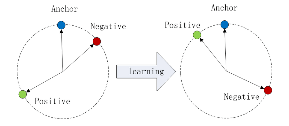
The distance from the anchor to the positive is minimized, and the distance from the anchor to the negative input is maximized.
-
Data
- Random Netgative
- The anchor and positive is usually collected from positive pairs (either by human labeling or by implicit data collection)
- Negative example is usually not explicitly collected, so random negative assignment is common.
- Since random negatives are often too easy to distinguish, after a few iterations, the model learns nothing.
- Online Negative Mining
- To resolve this problem, online negative mining look for hard negatives from the current batch, instead of using one initally assigned.
- Practically, large batch size is required for good performance, since there are few hard negative with small batch size. However, online negative mining takes time for k-NN.
- Semi-hard Negative Mining
- Always using the hardest negative can be dangerous. Hard negative can make to reduce , paying .
- So it is important to pick a negative whose current anchor-negative distance is just above the anchor-positive distance. (Semi-hard negative)
- Random Netgative
-
CDML (Collaborative Deep Metric Learning)
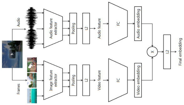
- CDML freezes feature extractor layers and trains embedding network with triplet loss

- Limitations
CDML requires a large batch size due to online negative mining.
17.3. Contrastive Learning
17.3.1. Pairwise Loss
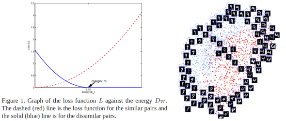
- For a pair of input examples, ground truth distance is either 0 (similar) or 1 (dissimilar).
- For each case, it applies different loss functions, (similar) or (dissimilar).
- is the distance between and computed by the model.
17.3.2. Negative Samping
- Softmax
- Cross-entorpy
- Only one term (where ) alives in cross-entropy, but softmax depends on all other probabilities due to the denominator.
- This makes the loss depend on every output in the network, which means every network parameter will have a non-zero gradient. So the model needs to update for every training example.
- Can we just sample some negatives, instead of computing all of them?
- For most irrelevant labels, .
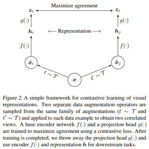
17.3.3. SimCLR (A Simple Framework for Contrastive Learning of Visual Representations)
-
Architecture
-
Loss
-
Self-supervised learning: no label is required.
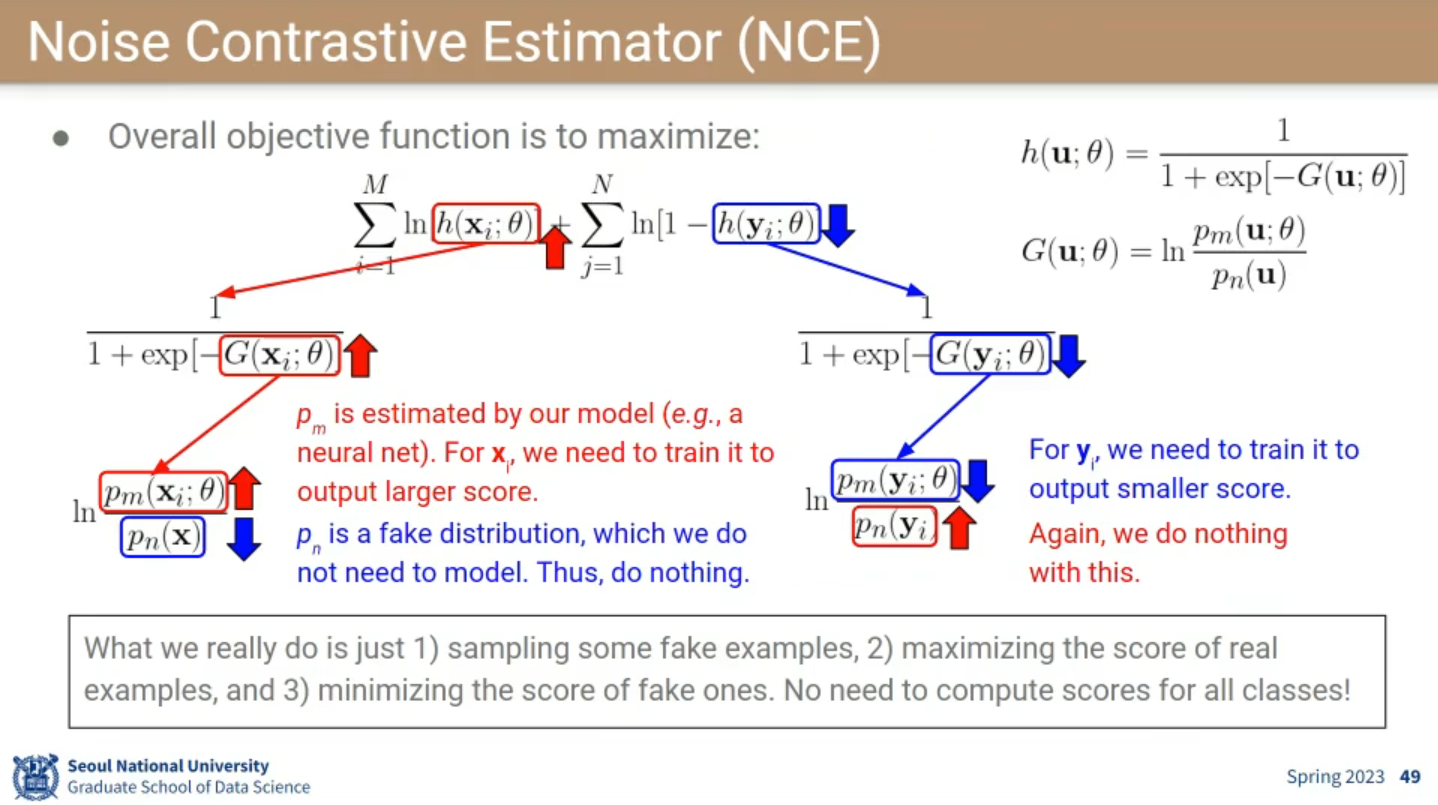
17.3.4. Noise Contrastive Estimator (NCE)
-
Idea
- examples from observed probability distribution
- examples from fake probability distribution , generated artificially
- Now, NCE trains the model to distinguish if each sample came from or .
- Binary classification task with logistic regression
- Summary
- Sample some fake examples
- Maximize the score of real examples
- Minimize the score of fake ones
- No need to compute scores for all classes
-
Loss
📙 강의
