14. Transformers Ⅱ
14.1. Transformer-based Image Models
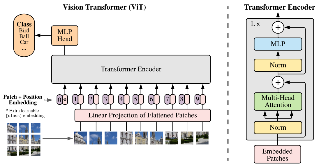
14.1.1. ViT (Vision Transformers)
-
The standard Transformer model is directly applied to images
- An image is split into patches. Each token is the patch instead of a word.
- The sequence of linear embeddings of these patches are fed into the Transformer.
- Eventually, an MLP is added on top of the [CLS] token to classify the input image.
-
Shape and Architecture
- image
- sequence of flattend 2D patches
- is the resolution of image patch.
- patch embedding
- trainable linear projection
- trainable linear projection
- positional embdding
- The MLP contains two layers with a GELU non-linearity.
- , (Multi-Head Self-Attention)
- image
-
Experiments and Discussion
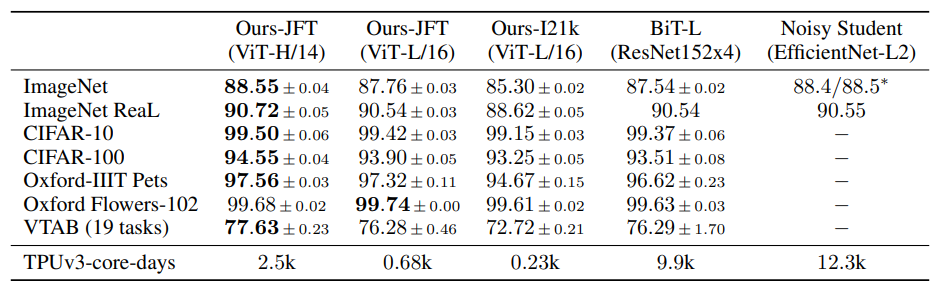
- ViT is computationally expensive. It takes 300 days with 8 TPUv3 cores.
- ViT performs well only when trained on an extremely large dataset. Why?

- ViT does NOT imply any inductive bias (spatial locality & positional invariance) of CNNs.
- So it requires large data to learn those purely from the data.
- However, with sufficient data, it can outperform CNN-based models, since it iis capable of modeling hard cases beyond spatial locality.
- Position embedding
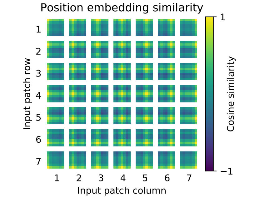
- Closer patches tend to have more similar position embeddings, automatically learned from data.
- ViT is computationally expensive. It takes 300 days with 8 TPUv3 cores.
14.1.2. DeiT (Data-efficient image Transformers)
-
Contributions
- ViT does not generalize well when trained on insufficient amounts of data.
→ DeiT uses Imagenet as the sole training set. - The training of ViT models involved extensive computing resources.
→ DeiT train a vision transformer on a single 8-GPU node in two to three days.
- ViT does not generalize well when trained on insufficient amounts of data.
-
Main idea: Distillation
-
Teacher model
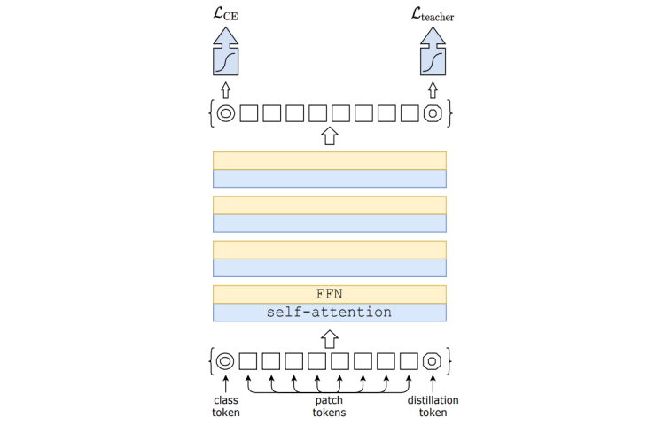
DeiT exploits strong image classifier as a teacher model to learn a transformer. DeiT simply includes a new distillation token. The distillation token interacts with the class and patch tokens through the self-attention layers. -
Soft vs. Hard distillation
- notations
- : teacher logits
- : student logits
- : temperature for the distillation
- : the Kullback-Leibler divergence loss
- : the softmax function
- : the hard decision of the teacher
- Soft distillation
- Hard-label distillation
- notations
-
Distillation token
-
-
Experiments and Discussion
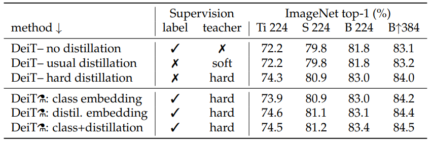
- Hard distillation (83.0%) significantly outperforms soft distillation (81.8%), even when using only a class token.
- The two tokens (class + distillation) is significantly better than the independent classifiers.
- The distillation token gives slightly better results than the class token probably due to the inductive bias of convnets.
14.1.3. Swin Transformer
-
Issues with Vanilla ViT Model
- Too much computational cost due to lack of inductive bias
- The model need to refer to all tokens in the image, even though in most cases only the nearby patches are informative.
- Fixed-size patches
- Variations in the scale of visual entities are not properly modeled.
- Pixels across patches cannot directly interact even though they are adjacent.
- Too much computational cost due to lack of inductive bias
-
Main idea
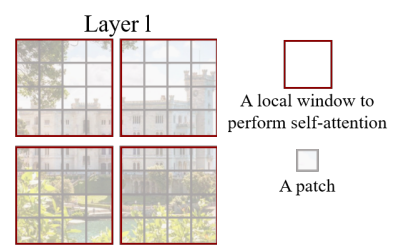
- Inductive Bias Reintroduced (by Self-attention in non-overlapped windows)
For efficient modeling, the model compute self-attention within local windows. The number of patches in each window is fixed.
- Time Complexity
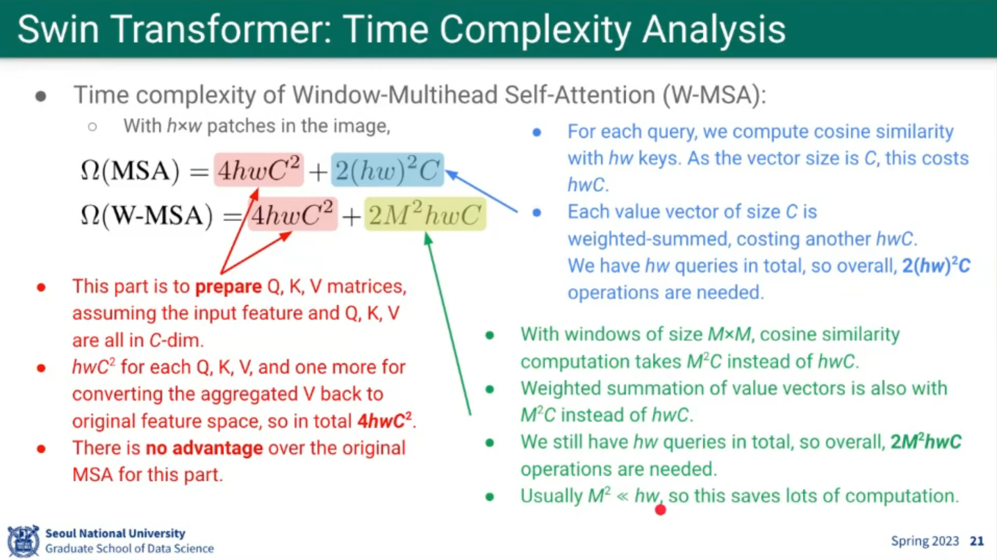
- Time Complexity
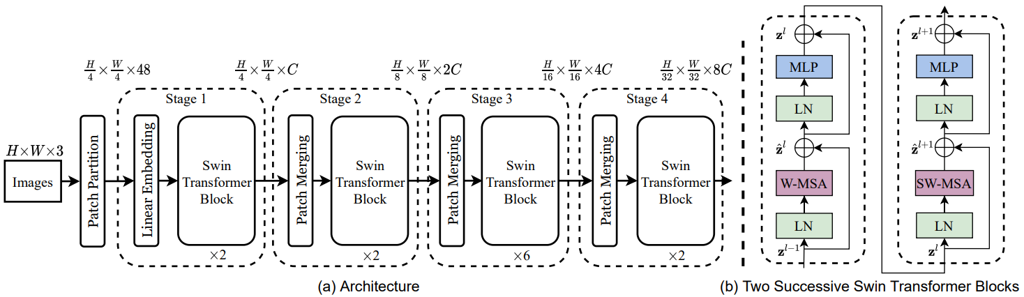
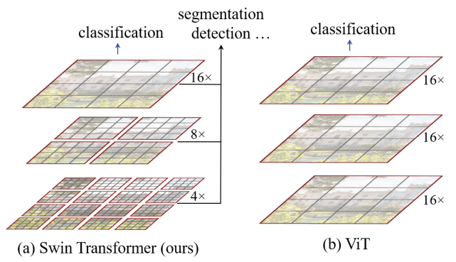
- Hierarchical Structure
The model constructs a hierarchical representation by starting from small-sized patches in deeper Transformer layers. To produce a hierarchical representation, the number of tokens is reduced by patch merging layers as the network gets deeper. It can serve as a general-purpose backbone for both image classification and dense recognition tasks.
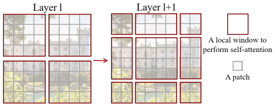
- Shifted Window (Swin) Partitioning
A key design element is shift of the window partition between consecutive self-attention layers. The shifted windows bridge the windows of the preceding layer, providing connections among them that significantly enhance modeling power.
- Relative Position Bias
Since only the patches within the window participate in self-attention, only the relative position bias within the window does matter.
- Inductive Bias Reintroduced (by Self-attention in non-overlapped windows)
14.1.4. CvT (Convolutional vision Transformers)
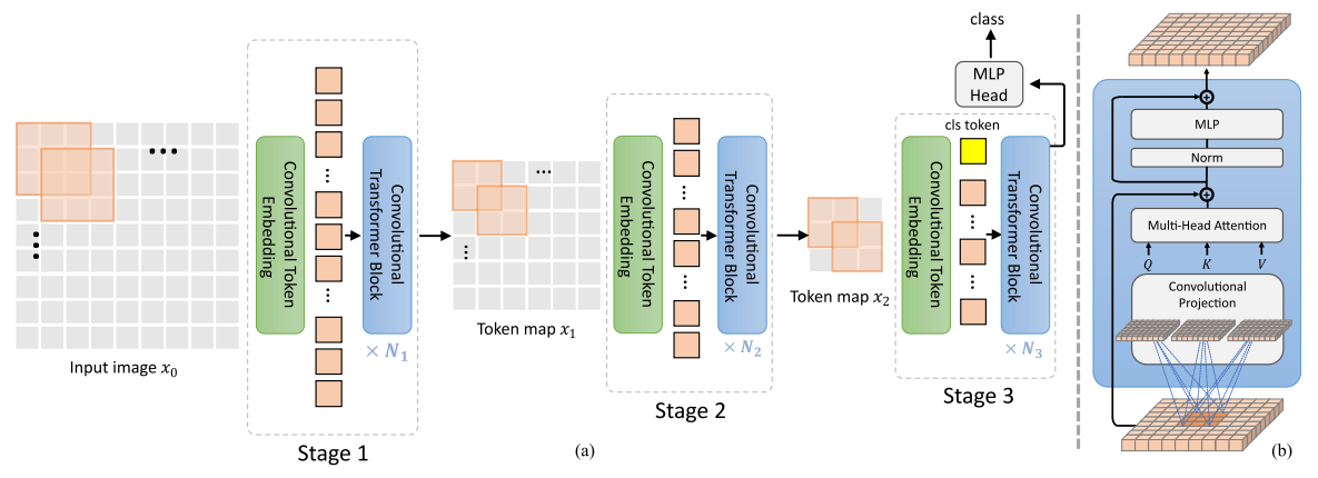
A multi-stage (3 in this work) hierarchy design borrowed from CNNs is employed. Each stage has two parts, Convolutional Token Embedding and Convolutional projection.
-
Issues with Vanilla ViT Model
- Too much computational cost due to lack of inductive bias
- The model need to refer to all tokens in the image, even though in most cases only the nearby patches are informative.
- Fixed-size patches
- Variations in the scale of visual entities are not properly modeled.
- Pixels across patches cannot directly interact even though they are adjacent.
- Too much computational cost due to lack of inductive bias
-
Main idea
-
Convolutional Token Embedding layer
- The layer is implemented as a convolution with overlapping patches with tokens reshaped to the 2D spatial grid as the input.
- The degree of overlap can be controlled via the stride length.
- These layers have the ability to represent increasingly complex visual patterns over increasingly larger spatial footprints, simliar to CNNs. Since
- each stage progressively reduce the number of tokens (i.e. feature resolution), thus achieving spatial downsampling.
- each stage progressively increase the width of the tokens (i.e. feature dimension), thus achieving increased richness of representation.
- Implementation
- Input to stage
- 2D image or 2D-reshaped output token map form a previous stage
- new tokens
- where is 2D conv operation
- channel size:
- kernel size:
- stride:
- padding: p
- The new token map
- height and width
- is then flattened into size
- height and width
- Input to stage
-
Convolutional projection
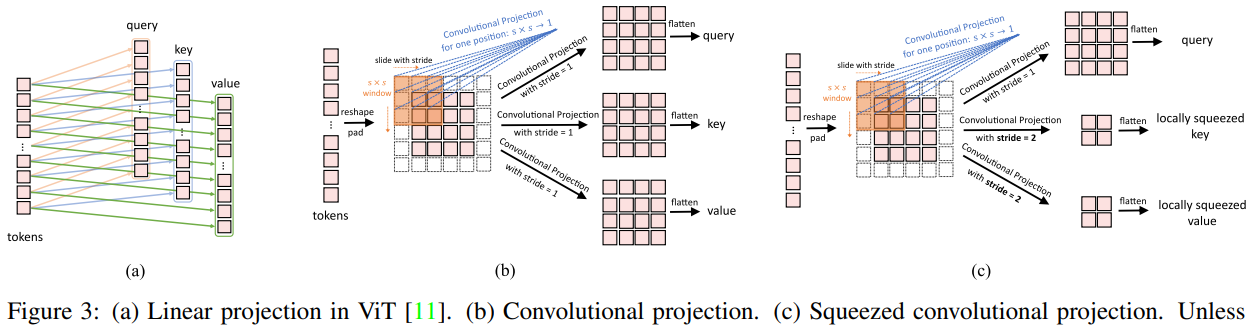
- Next, a stack of the proposed Convolutional Transformer Blocks comprise the remainder of each stage.
- A depth-wise separable convolution operation, referred as Convolutional Projection, is applied for query, key, and value embeddings respectively, instead of the standard position-wise linear projection in ViT.
- Convolutional Projcection
- is a depth-wise separable convolution implemented by:
- is a depth-wise separable convolution implemented by:
-
14.2. Transformer-based Video Models
14.2.1. ViViT (Video Vision Transformer)
-
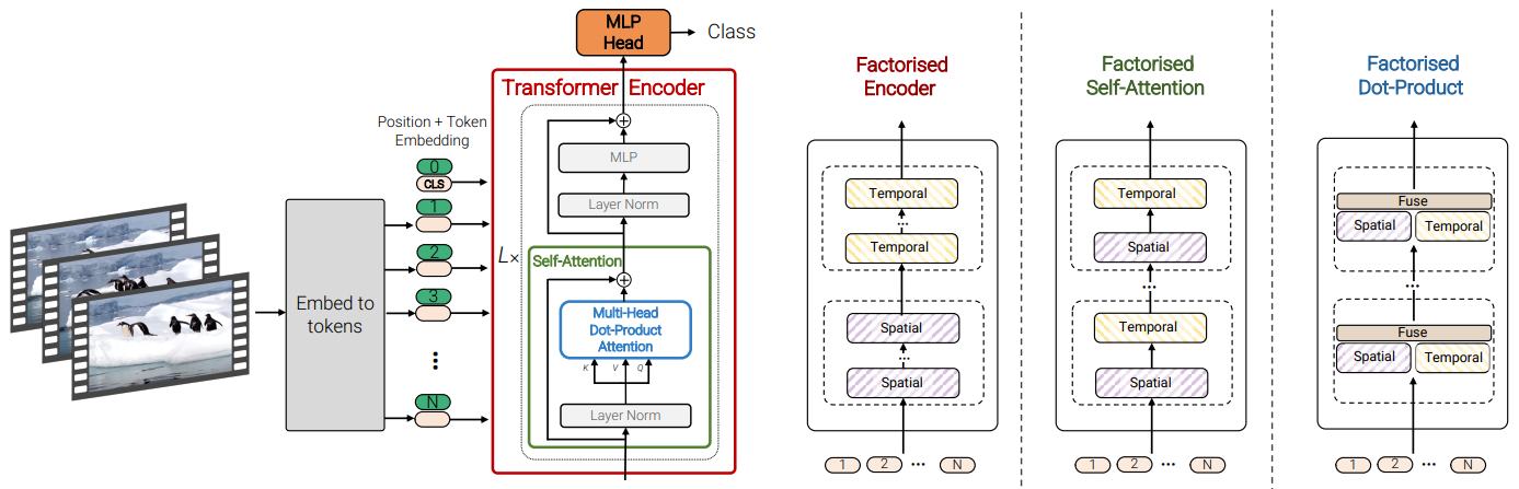
Model 1: Spatio-temporal attention
- Naturally extending the idea of ViT to video classification task
- Total patches are fed into the Transformer Encoder.
- Computationally expensive:
- Basic ideas to reduce computational overhead

- Basic ideas to reduce computational overhead
-
Model 2: Factorized encoder
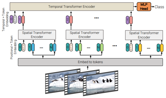
- First, Spatial Transformer Encoder (=ViT)
- Then, each frame is encoded to a single embedding and fed into the Temporal Transformer Encoder
- Complexity:
-
Model 3: Factorized self-attention
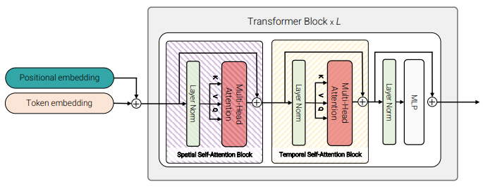
- First, only compute self-attention spatilally (among all tokens, extracted from the same temporal index)
- Then, temporally (among all tokens extracted from the same spatial index)
- No [CLS] is used to avoid ambiguities.
-
Model 4: Factorized dot-product attention
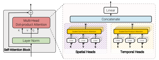
- Recall that the Transformer is based on Multi-head attentions.
- Half of the attention heads operate with keys and values from same spatial indices.
- The other half operate with keys and values from same temporal indices.
-
Experiments and Discussion
- Dataset sparsity problem
- ViT requires extremely large dataset.
- There's no large video dataset.
- Model 2 can be initialized with ViT.
- Comparing Model 1, 2, 3, 4
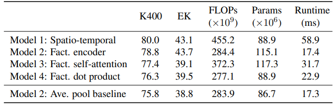
- The naive model (Model 1) performs the best, but most expensive.
- Model 2 is the most efficient.
- Dataset sparsity problem
14.2.2. TimeSFormer
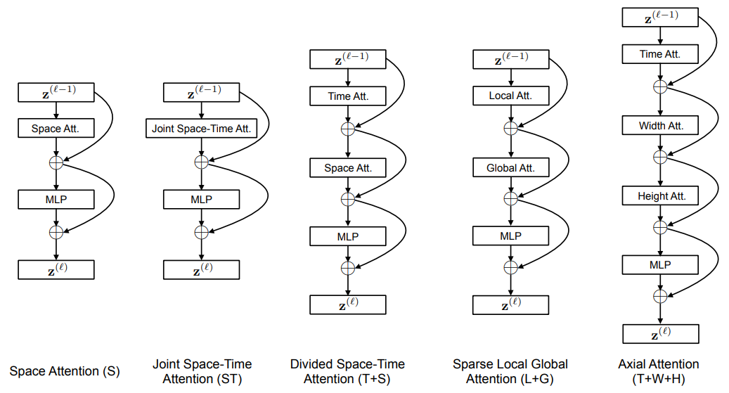
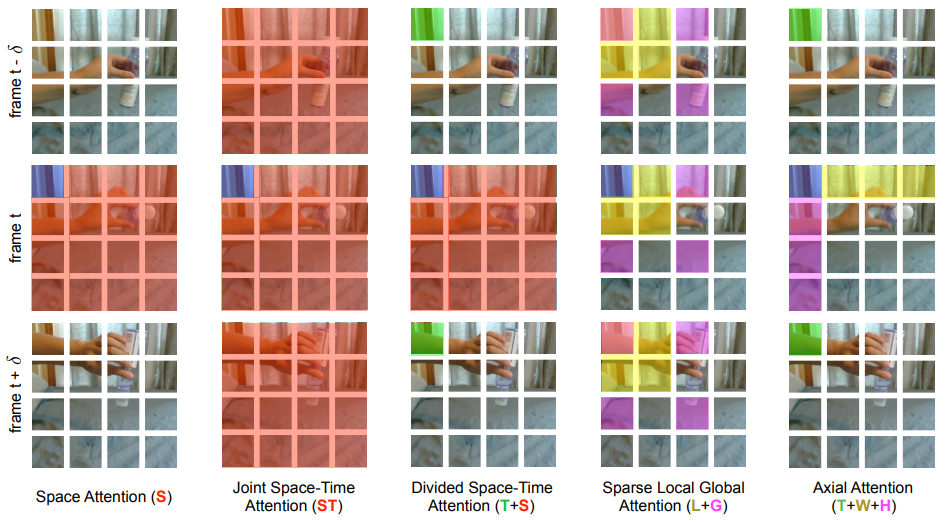
- (S) = ViT
- (ST) = ViViT Model 1
- (T+S) ViViT Model 3
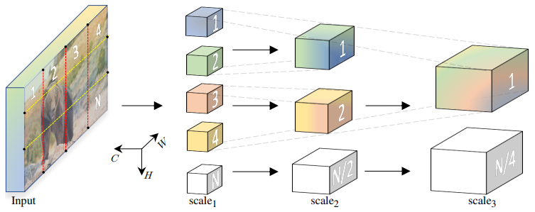
14.2.3. MViT (Multiscale Vision Transformers)
-
A similar idea to CvT, applied to videos.
-
Multi Head Pooling Attention (MHPA)
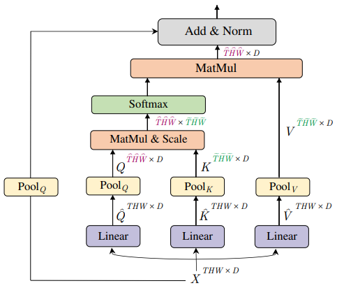
- Progressively pooling the resolution from input to output of the network, while expanding the channel capacity, following the widely-used paradigm with CNNs.
- Pooling layers reduce Time-Height-Width resolutions.
- Queires and keys/values are reduced to different sizes, similar principle to the squeezed convolutional projection in CvT.
-
Compared to CvT
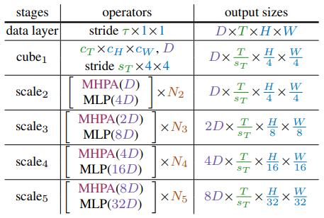
- cube corresponds to the first Conv Token Embedding layer.
- After then, MViT shrinks the feature map size by pooling operations within MHPA, not conv operations as in CvT.
- Recall that Conv Transformer Block in CvT self-contains MLP layers. This block is analogous to [MPHA; MLP] in MViT.
-
Discussion
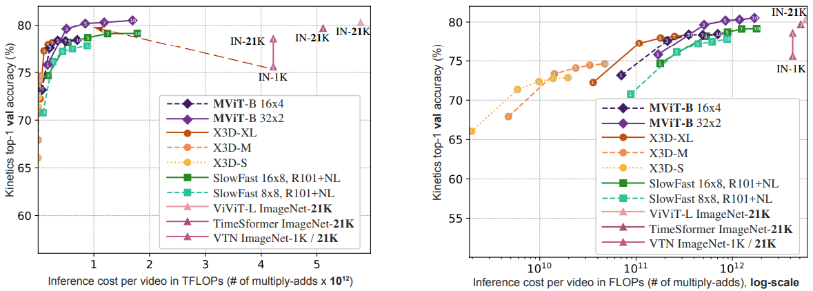
- Achieves slightly better performance than ViViT and TimeSformer, with significantly smaller inference cost.
- Comparing with CNN models:
- X3D model
- SlowFast model
14.3. Further Readings
- Video Transformers: A survey
- UniFormer: Unified Transformer for Efficient Spatiotemporal Representation Learning
- Self-supervised Video Transformer
- Vision Transformer with Deformable Attention
📙 강의
