R Girshick. Rich feature hierarchies for accurate object detection and semantic segmentation. CVPR 2014.

---

1. 문제 정의

2000년대 visual recognition은 SIFT와 HOG를 이용한 feature에 기반하였다. 2010~2012년에는 앙상블이나 기존 방법에서의 마이너한 변화를 통해 작은 개선만이 이루어졌다.

한편, LeNet을 비롯한 CNN은 1990년대에 활발히 이용되다가 SVM의 등장으로 인기가 식어 갔다. 그러다가 2012년에 AlexNet이 image classification에서 상당한 정확도를 기록함으로써, CNN이 다시 주목받게 되었다. 이는 CNN이 classification에서 object detection으로 어느 정도까지 일반화될 수 있는지에 대한 활발한 토론으로 이어졌다.

R-CNN은 image classification과 object detection의 gap을 줄이고 싶었고, CNN이 object detection에서 높은 성능을 낼 수 있음을 처음으로 증명하였다. R-CNN은 이를 위해 두 가지 문제에 집중하였다. 첫 번째는 deep network로 objects를 localizing하는 것, 두 번째는 적은 양의 데이터로 큰 모델을 학습시키는 것이다.

1.1. Localizing objects with a deep network

image에서 objects를 localizing하는 문제에는 기존에 두 가지 접근법이 존재하였다. 하나는 localization을 regression으로 푸는 것이다. 그러나 이는 현실과 잘 맞지 않았다 (당시 VOC 2007에서 이 방법은 30.5%, R-CNN은 58.5%를 기록). 다른 하나는 sliding window 방식이다. R-CNN도 이 방식을 적용해 보았다. 하지만 AlexNet 구조를 이용한 R-CNN은 다섯 개의 convolution layer로 인해 receptive fileds ($195 \times 195$)와 strides ($32 \times 32$)가 컸고, 때문에 정확인 localization이 어려웠다.

대신 R-CNN은 selective search를 이용한 "recognition using regions"로 문제를 해결하였다. selective search는 아래 2.1.에 간단히 설명하였다.

1.2. Training a large CNN when data is scarce

또 다른 문제는 labeled data가 적을 때 큰 CNN을 학습시키는 것이었다. 기존에는 unsupervised pre-training으로 feature를 학습한 뒤, supervised fine-tuning을 하는 것이 해결책이었다. 그러나 R-CNN은 많은 데이터를 사용한 supervised pre-training과 적은 데이터를 사용한 domain-specific fine-tuning이 좋은 성능을 낼 수 있음을 증명하였다.

---

2. Module Design

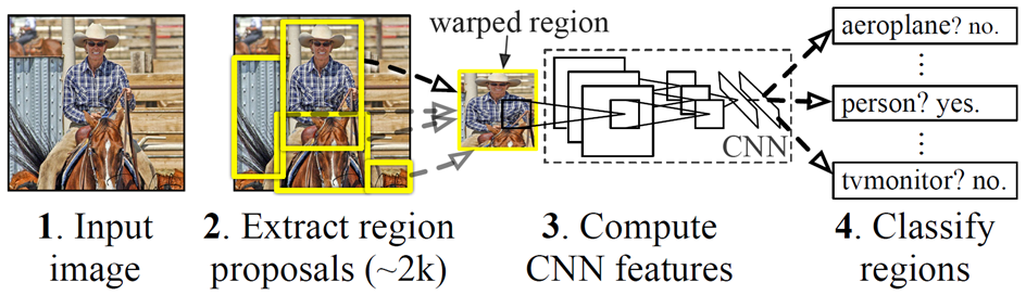
1) 약 2000개의 region proposals를 추출
2) CNN을 이용해 각 proposal로부터 고정된 크기의 feature vector를 계산
3) category-specific SVM으로 2)의 vector를 분류
4) 2)의 vector로부터 bounding box를 regress
(Test-time에는 NMS를 적용)

2.1. Region Proposals

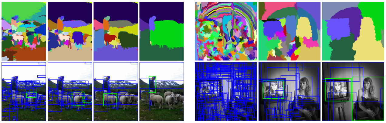
R-CNN의 첫 번째 단계는 selective search를 이용한 region proposals 추출이다. 위 그림은 selective search의 예이다. selective search는 아래 식과 같이 두 regions의 색상, texture, 크기, fill을 이용해 유사도를 계산하여 모든 scale에서 merge를 반복함으로써 region proposals를 생성한다 (알고리즘과 각 요소의 자세한 식은 selective search 논문 참조).

2.2. Feature Extraction (CNN)

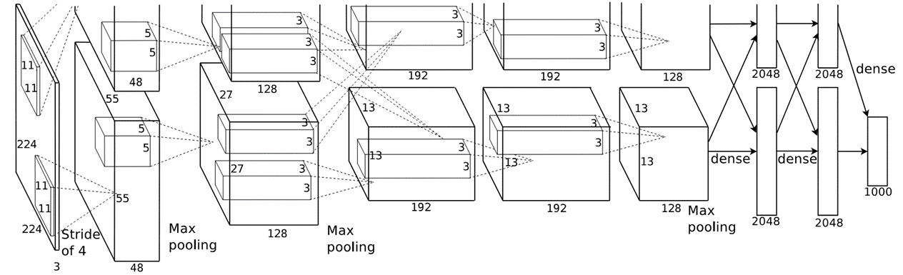
R-CNN은 CNN을 사용해 각 region proposal로부터 4096-d의 feature vector를 계산하였다. CNN 구조로는 위 그림의 AlexNet을 사용하였다. AlexNet은 5개의 convolutional layers와 2개의 fc layers로 이루어져 있다.

2.2.1. Warping

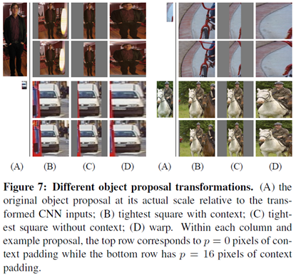
AlexNet은 고정된 크기인 $227 \times 227$을 input으로 받기 때문에 크기가 arbitrary한 각 region proposal의 크기도 이에 맞추어야 했다. 논문은 위 그림처럼 여러 가지 방법을 시도해 보았고, 가장 성능이 좋았던 warp + padding ($p = 16$)을 사용하였다.

2.2.2. Supervised Pre-training

큰 CNN을 학습하기에는 당시 object detection 데이터가 적었기 때문에, R-CNN은 supervised pre-training을 이용하였다. 상대적으로 데이터가 많은 image classification task의 ILSVRC2012 데이터를 이용하여 feature를 충분히 학습하였다.

2.2.3. Domain-specific Fine-tuning

• The Last FC Layer
  pre-train된 CNN parameter를 detection task에 맞추기 위해 fine-tuning이 필요하였다. 이를 위해 위에서 소개한 AlexNet의 마지막 fc layer를 $1000$-way에서 ($N+1$)로 변경하여 전체 network의 fine-tuning을 진행하였다 ($N$은 object class 수, $1$은 background).

• Positive vs. Negative
  region proposals 중 ground-truth와 $0.5$ 이상의 $\mathrm{IoU}$를 가지는 경우를 gt class의 positive로, 나머지는 negative로 분류하여 학습을 진행하였다.

  (Appendix B 내용)
  이때 gt가 아닌, $0.5$와 $1$ 사이의 $\mathrm{IoU}$를 가지는 region proposals를 사용함으로써 "jittering" 효과를 주게 되었다. 이는 positive examples의 수를 30배 가까이 늘려주었기 때문에 전체 network의 overfitting을 방지했을 것으로 추측하였다. 그러나 이 jittered examples는 정확한 localization을 위한 fine-tuning에는 최적의 방법이 아닐 것이다. 이는 SVM의 fine-tuning에 다른 기준을 사용한 것으로 이어지게 된다.

• Learning Rate
  pre-train된 parameter의 지나친 수정을 피하기 위해 pre-training rate의 $1 \over 10$ 크기인 $0.001$을 learning rate로 SGD 학습을 시작하였다.

• Batch
  각 배치마다 모든 classes에서 32개의 positive region proposals와 96개의 background (negative) region proposals를 sampling하였다. positive가 background에 비해 extremely rare하였기 때문이다.

2.2.4. Object Category Classifiers

• Positive vs. Negative
  ground-truth만을 그 class의 positive로, gt와 $0.3$ 이하의 $\mathrm{IoU}$를 가지는 region proposals를 negative로 분류하여 SVM의 학습을 진행하였다. $0.3$보다는 크지만 gt가 아닌 proposals는 무시하였다.

  (Appendix B 내용)
  object detector로 softmax classifier를 사용해도 되었을 텐데 SVM을 다시 학습한 이유가 있다. 성능 차이다 (50.9% vs. 54.2% mAP). 이렇게 차이가 나는 이유를 두 가지로 분석하였다. 첫 번째는 fine-tuning에 사용된 "jittered" positive examples는 정확한 localization에 방해가 되기 때문이다. 두 번째는 SVM은 softmax에 비해 "hard negatives"를 학습하였기 때문이다(hard negative mining method를 사용).

2.2.5. Bounding-Box Regression

localization errors를 줄이기 위해 class-specific bbox regressor를 사용하였다. region proposal이 다섯 번째 conv layer를 통과한 이후 max-pooling된 pool$_5$ features를 이용하여 새로운 detection window를 예측하였다. 이로써 mAP를 3~4 points 상승시키는 효과를 가져왔다.

• Input
  $N$개의 training pairs $\{(P^i, G^i)\}_{i=1, ..., N}$

  여기서 $P^i = (P^i_x, P^i_y, P^i_w, P^i_h)$는 proposal $P^i$ bbox의 pixel 단위 center, 넓이, 높이이고, $G^i$는 ground-truth이다.

  gt와 $0.6$ 이상의 $\mathrm{IoU}$ 값을 가지는 proposal만을 사용하였다.

• Transformation
  $P$를 $G$로 mapping하기 위한 4개의 함수 $d_x(P)$, $d_y(P)$, $d_w(P)$, $d_h(P)$를 parameterize하였다. $d_x(P)$, $d_y(P)$는 center에 대한 scale-invariant translation, $d_w(P)$, $d_h(P)$는 넓이와 높이에 대한 log-space translation이다. 이 함수들을 학습한 뒤에 아래와 같이 input proposal $P$를 predicted gt bbox $\hat{G}$로 transform할 수 있다.

  $\hat{G}_x = P_w d_x(P) + P_x \\ \, \\ \hat{G}_y = P_h d_y(P) + P_y \\ \, \\ \hat{G}_w = P_w \, \mathrm{exp}(d_w(P)) \\ \, \\ \hat{G}_h = P_h \, \mathrm{exp}(d_h(P))$

• Function $d_*(P)$

  $d_*(P) = \mathrm{w}_*^\intercal \phi_5(P)$

  여기서 $\phi_5(P)$는 proposal $P$의 pool$_5$ features이고, $\mathrm{w}_*$는 learnable model parameters이다.

• Regression targets $t_x$

  $t_x = (G_x - P_x) / P_w \\ \, \\ t_y = (G_y - P_y) / P_h \\ \, \\ t_w = \log{(G_w / P_w)} \\ \, \\ t_h = \log{(G_h / P_h)}.$

• Optimizing $\mathrm{w}_*$
  아래와 같이 ridge regression을 사용하였으며, $\lambda$는 $1000$으로 설정하였다.

  $\mathrm{w}_* = \underset{\hat{\mathrm{w}}_*}\mathrm{argmin} \sum_i^N{(t_*^i - \hat{\mathrm{w}}_*^\intercal \phi_5(P^i))^2 + \lambda \lVert \hat{\mathrm{w}}_* \rVert^2}$
  • e. g.
    $\mathrm{w}_x = \underset{\hat{\mathrm{w}}_x}\mathrm{argmin} \sum_i^N{(t_x^i - \hat{\mathrm{w}}_x^\intercal \phi_5(P^i))^2 + \lambda \lVert \hat{\mathrm{w}}_x \rVert^2} \\ \, \\ = \underset{\hat{\mathrm{w}}_x}\mathrm{argmin} \sum_i^N{(t_x^i - d_x(P^i))^2 + \lambda \lVert \hat{\mathrm{w}}_x \rVert^2} \\ \, \\ = \underset{\hat{\mathrm{w}}_x}\mathrm{argmin} \sum_i^N{[(G_x^i - \hat{G_x^i} / P_w^i)]^2 + \lambda \lVert \hat{\mathrm{w}}_x \rVert^2}$
    $\mathrm{w}_h = \underset{\hat{\mathrm{w}}_h}\mathrm{argmin} \sum_i^N{(\log{G_h^i} - \log{\hat{G_h^i}})^2 + \lambda \lVert \hat{\mathrm{w}}_h \rVert^2}$

---

3. Experiments

3.1. Results on VOC 2010

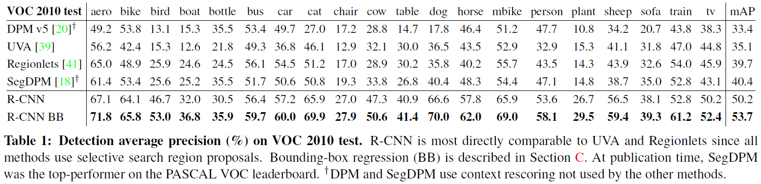
여러 methods 가운데 R-CNN이 가장 높은 mAP를 기록하였다. 같은 region proposal 알고리즘을 사용한 UVA가 가장 밀접한 관련이 있다.

3.2. Results on ILSVRC2013 detection

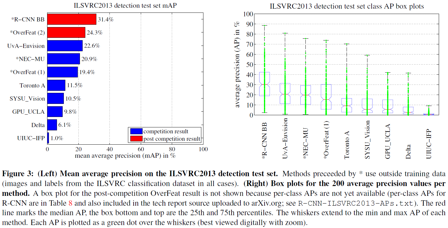
여러 methods 중 R-CNN이 가장 높은 mAP를 기록하였다. 오른쪽 box plot을 보면 각 클래스별 AP 역시 R-CNN이 전체적으로 높은 것을 확인할 수 있다.

3.3. Ablation Studies

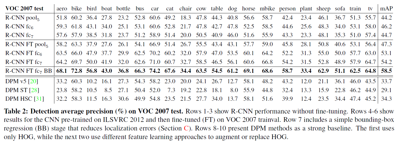
• without fine-tuning
  fc$_7$이 fc$_6$보다 나쁜 결과를 기록하였다. 이는 mAP의 하락 없이 16.8m개(29%)의 CNN parameters가 제거될 수 있음을 의미한다. 또한 pool$_5$가 CNN parameters의 6%만을 사용함에도 불구하고 fc$_6$과 fc$_7$이 없이 꽤 괜찮은 결과를 기록하였다. 즉, CNN의 representational power 대부분은 훨씬 큰 계산 규모를 가지는 fc layers에서보다 conv layers에서 온다.

• with fine-tuning
  fine-tuning으로 mAP를 46.2에서 54.2까지 8% 포인트 향상시켰다. fine-tuning으로 인한 상승은 pool$_5$보다 fc$_6$와 fc$_7$에서 더욱 컸다. 이는 ImageNet으로 pre-training된 pool$_5$ features가 충분히 general하며, 정확도 향상의 대부분은 domain-specific non-linear classifier에서 비롯되었음을 의미한다.

• vs. recent feature learning methods
  모든 R-CNN variants가 3개의 DPM baselines를 크게 앞질렀다.

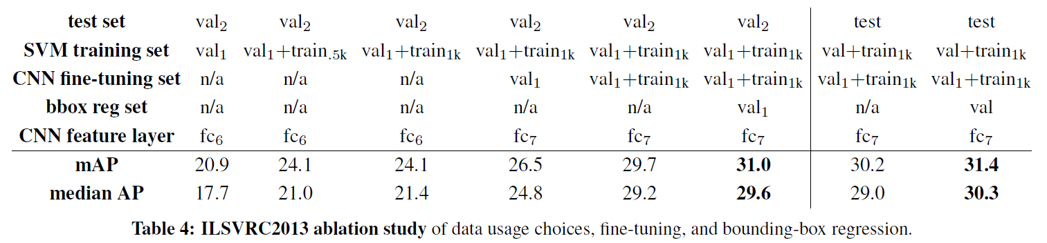
• on ILSVRC2013 detection
  더 많은 데이터, fine-tuning, bbox regressor가 mAP를 향상시켰다.

3.4. Network Architectures

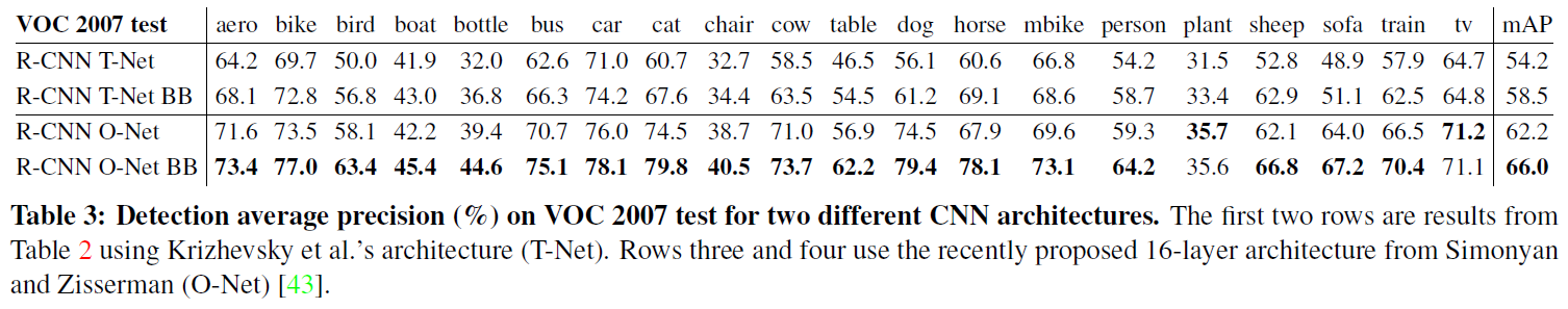
T-Net은 AlexNet, O-Net은 VGGNet을 가리킨다. 더 깊은 구조인 VGGNet이 mAP를 크게 끌어올렸지만, computing time이 AlexNet보다 7배 더 오래 걸린다는 단점이 있었다.

3.5. Error Analysis

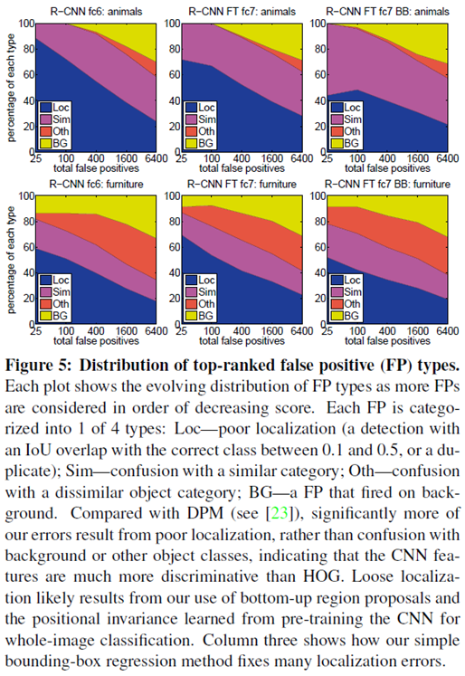
DPM과는 달리 Error의 대부분이 객체와 배경의 confusion보다는 localization에서 발생하였다. 이는 CNN features가 HOG보다 더욱 discriminative함을 의미한다. localization errors는 region proposals와, image classification으로 pre-training된 CNN의 positional invariance로부터 발생한 것으로 보인다. bbox regression이 이러한 localization errors를 효과적으로 fix하였다.

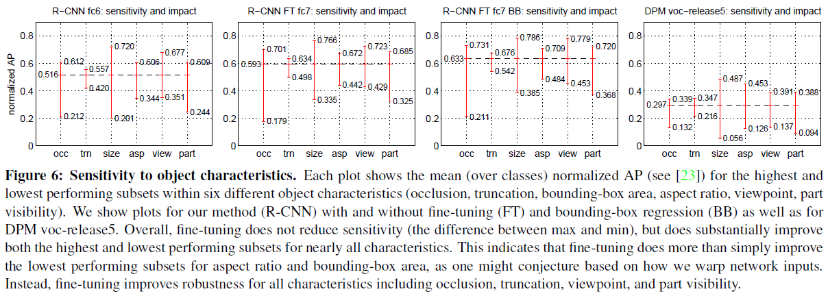
fine-tuning이 object 특징별 mAP의 sensitivity를 줄이지는 않았지만, 전체적으로 mAP를 향상시켰다. 이는 fine-tuning이 모든 특징에서 robustness를 가져다주었음을 의미한다.

3.6. Bounding-Box Regression

위에서 소개한 여러 결과에서 bbox regression을 사용하였을 때 정확도가 크게 향상되었다.

---

4. Conclusion

Object detection의 performance는 당시 몇 년간 정체되어 있었으나, R-CNN은 간단히 적용할 수 있는 알고리즘으로 결과를 30% 가까이 향상시켰다. R-CNN은 두 insights를 통해 이를 이뤄낼 수 있었다. 첫 번째로, 객체의 localization과 segmentation을 위해 region proposals에 큰 CNN을 적용하였다. 두 번째로, 데이터가 적을 때 큰 CNN을 학습하는 방법이다. 충분한 데이터로 pre-train한 뒤, target task의 적은 데이터로 fine-tuning하는 것이다. 즉 "supervised pre-training/domain-specific fine-tuning"이다. R-CNN은 고전적인 computer vision과 딥러닝을 결합하여, 이 둘이 opposite이 아닌 inevitable partners임을 보여 주었다.