K He. Deep Residual Learning for Image Recognition. CVPR 2016.

---

1. 문제 정의

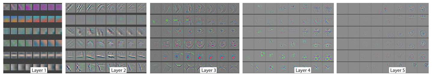
깊은 네트워크는 위 그림과 같은 low/mid/high-level features를 잘 통합한다. 그리고 features의 levels는 깊어질수록 풍부해진다. 당시 ImageNet dataset challenge에서 선두 그룹은 모두 "very deep"한 모델들을 사용하였다. 신경망의 깊이가 깊어질 경우 vanishing/expolding gradients 문제가 수렴을 방해하지만, 이 문제는 weight initialization과 batch normalization을 통해 대체로 해소되었다.

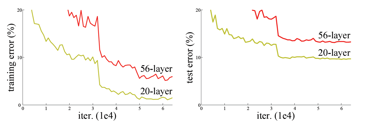
그러나 깊은 신경망이 수렴하기 시작한 뒤에는, 깊이가 깊어질수록 정확도가 saturate되었다가 급격하게 degrade되었다. 이를 degradation problem이라고 한다. 이 문제는 overfitting 때문이 아니다.

한 번 생각해 보자. identity mapping (입력=출력)인 layers를 shallower model의 끝에 추가하는 경우, 적어도 더 높은 training error가 나와서는 안 될 것이다. 그러나 multiple nonlinear layers로 이러한 identity mappings를 approximate하는 것에 어려움을 겪었기 때문에, ResNet 이전에는 이미 충분히 깊은 모델에 layers를 추가하는 경우 training error가 높아졌다.

ResNet은 이러한 degradation problem을 해결하기 위해 deep residual learning을 도입하였고, 이를 통해 더 깊은 신경망으로 더 좋은 성능을 얻을 수 있게 되었다.

---

2. Residual Learning

우리가 원하는 underlying mapping을 $\mathcal{H}(\mathrm{x})$라고 하자. 이 $\mathcal{H}(\mathrm{x})$에 $\mathrm{x}$를 빼줌으로써 $\mathcal{F}(x) := \mathcal{H}(\mathrm{x}) - \mathrm{x}$인 residual mapping을 정의할 수 있고, 우리는 nonlinear layers를 쌓음으로써 이 residual mapping을 fit하고자 한다. 여러 개의 nonlinear layers가 복잡한 함수인 $\mathcal{H}(\mathrm{x})$를 approximate할 수 있다면 (딥러닝의 기본 원리), 이 residual mapping도 approximate할 수 있을 것이다.

$\mathcal{H}(\mathrm{x})$를 optimzie하는 것보다 $\mathcal{F}(\mathrm{x})$를 optimize하는 것이 더 쉬울 것이다. 왜냐하면 identity mapping이 optimal인 경우, 여러 개의 nonlinear layers를 통해 $\mathcal{H}(\mathrm{x})$를 identity mapping으로 fit하는 것보다는 residual mapping인 $\mathcal{F}(\mathrm{x})$를 0으로 push하는 것이 더 쉬울 것이기 때문이다.

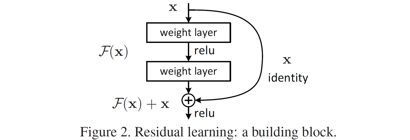
2.1. Building Block

• $\mathcal{F}(\mathrm{x}, \{W_i\})$는 학습되어야 할 residual mapping이다.

  • e. g. $\mathcal{F} = W_2 \sigma(W_1 \mathrm{x})$ where $\sigma$ denotes ReLU.
  • $\mathcal{F} + \mathrm{x}$는 element-wise addition이며, 무시해도 될 정도의 computational cost이다.
  • 두 번째 nonlinearity는 addition 이후에 적용한다.

• extra-parameter나 computation complexity가 추가되지 않는다.

• $\mathcal{F}$의 형태는 flexible하다. (논문은 2~3개의 layers 사용)

• $\mathrm{x}$와 $\mathcal{F}$의 차원이 맞지 않는 경우

  • Option (A): Zero-padding

    • 기본적으로 identity mapping을 적용하고, 늘어난 차원에서만 zero-padding을 적용한다.

  • Option (B): Linear projection

    $\mathrm{y} = \mathcal{F}(\mathrm{x}, \{W_i\}) + W_s \mathrm{x}.$
    • $1 \times 1$ convolution인 $W_s$를 이용해 맞춰준다.

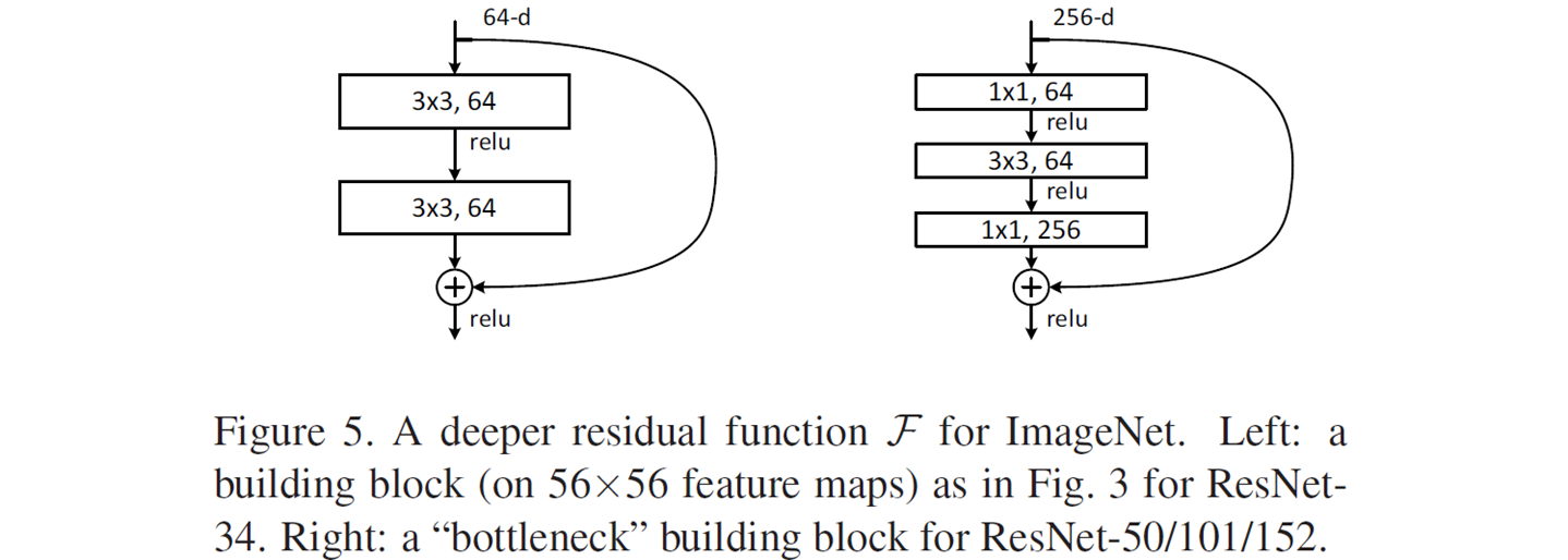
2.2. Bottleneck Building Block

• $1 \times 1$ layers가 $3 \times 3$ layer의 앞에서 차원을 줄이고 뒤에서 차원을 복원함으로써, $3 \times 3$ layer가 작은 input/output 차원을 갖는 bottleneck 모양이 된다.

• 아주 깊은 구조에서 affordable한 학습 시간을 위해 적용한다 (논문의 경우 50/101/152 layers에 적용). 위 그림의 두 block은 비슷한 time complexity를 가진다. 아래와 같이 실제로 계산하여 확인해 보았다.

  • Left: $56 \times 56 \times 64 \times 3 \times 3 \times 64 + 56 \times 56 \times 64 \times 3 \times 3 \times 64 = 231$m

  • Right: $56 \times 56 \times 64 \times 1 \times 1 \times 256 + 56 \times 56 \times 64 \times 3 \times 3 \times 64 + 56 \times 56 \times 256 \times 1 \times 1 \times 64 = 218$m

---

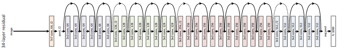
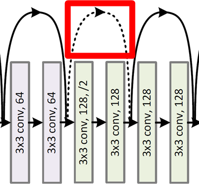
3. Network Architectures

• ResNet-34.
  

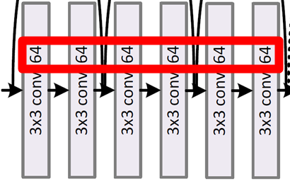
  • For the same output feature map size, the layers have the same # filters.
    

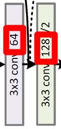
  • If feature map size is halved, # filters is doubled to preserve the time compelxity.
    

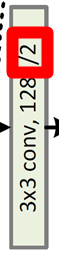
  • Downsampling by convolution layers with stride of 2.
    

  • Global average pooling layer.

  • 1000-way (# classes) fully-connected layers with softmax.

  • input/output 차원이 다른 경우, 2.1에서 소개한 option (A)나 (B)를 적용한다.
    

• Architectures for ImageNet.
  

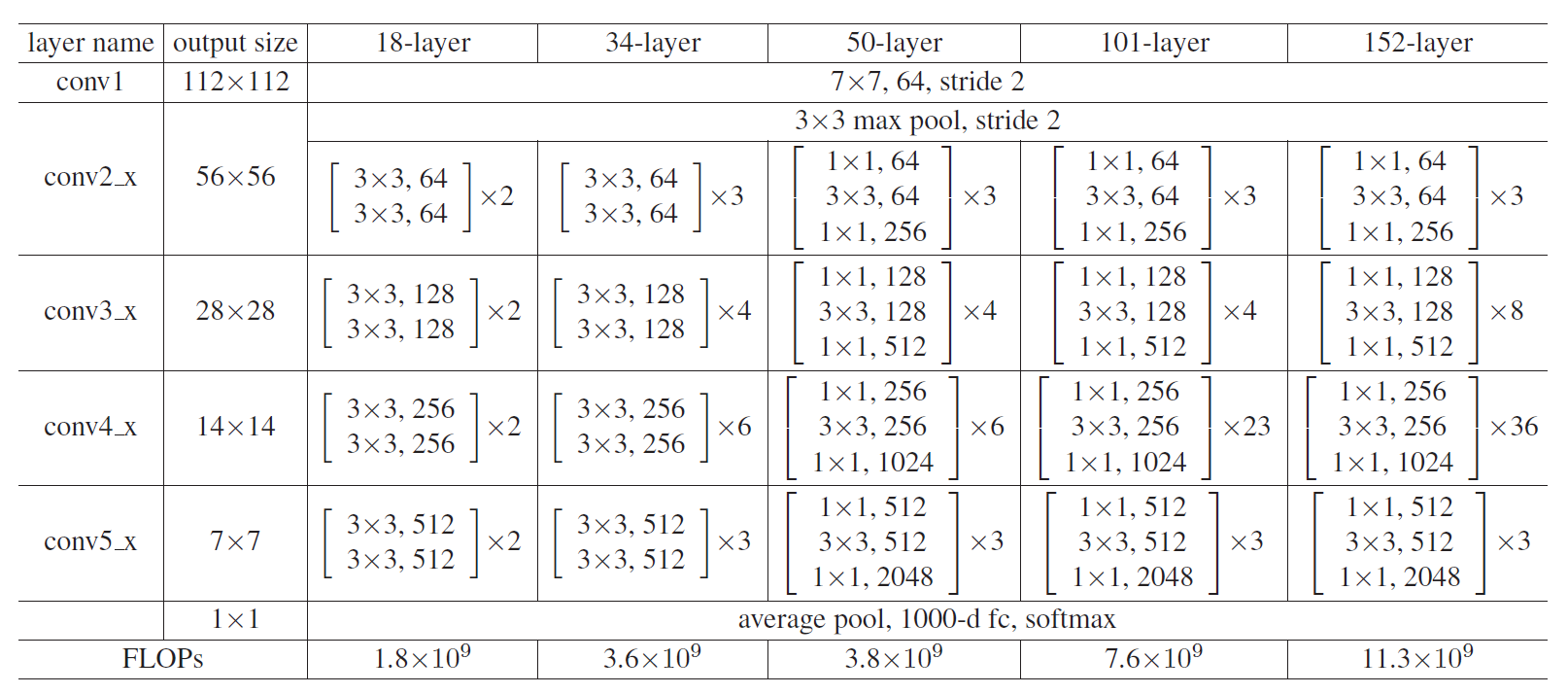
  • 50/101/152-layer에는 bottleneck building block이 사용되었다.

---

4. Experiments

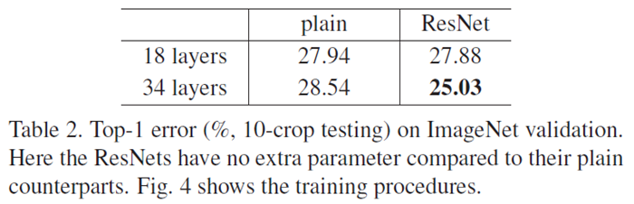
4.1. Plain vs. ResNet

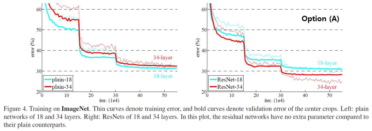
왼쪽은 plain network, 오른쪽은 shortcut을 활용한 residual network이다.

plain network의 경우, 더 깊은 34-layer의 validation error가 더 높았다. batch normalization을 적용했기 때문에, vanishing gradients가 이러한 degradation problem의 원인으로 보이지는 않는다.

우리는 그림과 표를 통해 세 가지의 주요한 관찰을 할 수 있다.

• (1) accuracy gains from increased depth.

  • plain network는 깊이가 깊어지는 경우 degradation problem으로 인해 정확도가 감소했다. 반면, ResNet은 깊이가 깊어지는 경우 정확도가 증가했다.

• (2) the effectiveness of residual learning on extremely deep systems.

  • 18-layers보다 34-layers에서 plain과 ResNet의 격차가 더욱 컸다. 깊어질수록 ResNet의 효과가 강해졌다.

• (3) 18-layers are comparably accurate, but ResNet converges faster.

  • 18-layers에서는 plain과 ResNet의 정확도가 비슷하지만, 그림에서 볼 수 있듯이 ResNet의 수렴 속도가 더욱 빨랐다.

4.2. Deeper ResNet

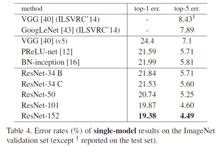
• ResNet은 깊어질수록 더욱 정확했다.

• 그럼에도 여전히 VGG-16보다 lower complexity를 가진다.

  Model	FLOPs (billon)
  ResNet-34	3.6
  ResNet-152	11.3
  VGG-16	15.3
  VGG-19	19.6

4.3. Closer to zero

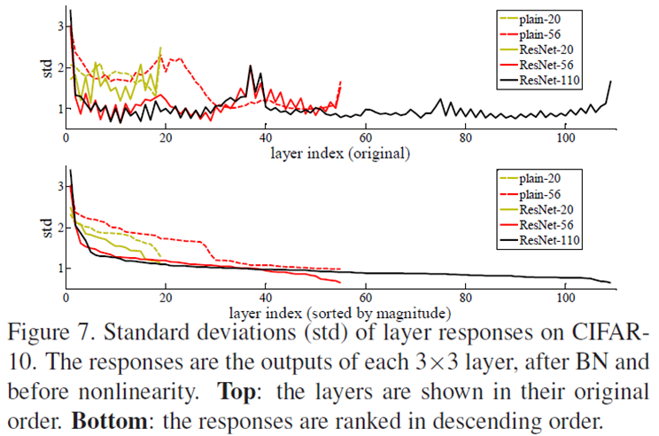
$3 \times 3$ layer의 outputs의 표준편차를 나타낸 그림이다 (batch normalization 이후, ReLU 이전). ResNet은 plain보다 작은 값들을 가졌고, 이것은 처음에 가정했던 대로 residual functions가 non-residual functions보다 0에 가깝다는 것을 의미한다.

4.4. Overfitting

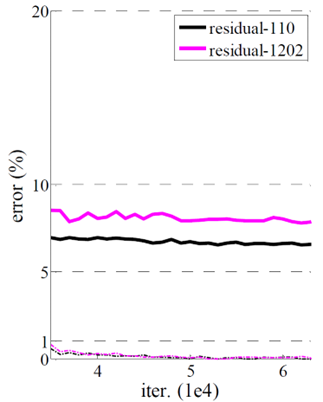
ResNet이더라도 데이터셋에 비해 깊이가 과도하게 깊어지는 경우, overfitting으로 인해 testing error가 높아지게 된다 (그림에서 training error는 비슷함).

---

5. Conclusion

ResNet은 multiple nonlinear layers에 shortcut connections를 추가하는 residual block을 활용함으로써 Deep Residual Learning을 구현하였고, 이를 통해 모델의 깊이가 깊어지는 경우 정확도가 감소했던 degradation problem을 효과적으로 해결하였다. 또한 ResNet은 깊은 구조일수록 더욱 효과적이었으며, 얕은 구조이더라도 plain의 경우보다 더욱 빠르게 수렴하였다. 한편, 모델의 깊이가 깊어지더라도 bottleneck building block을 활용하여 연산량을 줄일 수 있었다.

---

6. 구현 코드

PyTorch source code를 참고하여 논문에서 사용한 CIFAR-10 ResNet-20을 직접 구현하였다.

• per-pixel mean subtraction 미적용
• option (B) shortcuts 적용 (논문은 (A) 적용)