로지스틱 회귀

로지스틱 회귀

• 반응 변수가 범주형인 경우에 적용하는 회귀 분석을 로지스틱 회귀 분석이라 한다.
• 반응변수 Y를 직접 모델링 하지 않고 Y가 특정 범주에 속하는 확률을 모델링 한다.

import pandas as pd
import numpy as np
## 데이터 로드
body=pd.read_csv('./data/bodyPerformance.csv')
body

## binary 형태로 데이터 변환
## 이진 분류 형태로 전처리
body['gender']=np.where(body['gender']=='M', 0, 1)
body['class_1']=np.where(body['class']=='A', 1, 0)
body

from sklearn.model_selection import train_test_split

feature_columns = list(body.columns.difference(['class', 'class_1']))
x=body[feature_columns]
y=body['class_1']

train_x, test_x, train_y, test_y=train_test_split(x,y,stratify=y, train_size=0.7, random_state=1)
print(train_x.shape, test_x.shape, train_y.shape, test_y.shape)

### logisticRegression

from sklearn.linear_model import LogisticRegression
logR=LogisticRegression()
logR.fit(train_x, train_y)

## 확률 추정 로그 예측
proba=pd.DataFrame(logR.predict_proba(train_x))
## confidence score 구하기 x=0인 Hyperplane을 기준으로 양수/음수에 위치하는지 얼만큼 떨어져있는지
cs=logR.decision_function(train_x)

df=pd.concat([proba, pd.DataFrame(cs)], axis=1)
df.columns=['Not A','A', 'decision_function']

df.sort_values(['decision_function'], inplace=True)
df.reset_index(inplace=True, drop=True)

df

import matplotlib.pyplot as plt
## confidence score 에 따른 클래스 확률값을 매칭시키면 A 클래스에 
# 속한 추정확률과 결정경계를 얻을수 있다. 
plt.figure(figsize=(15,5))

plt.axhline(y=0.5, linestyle='--', color='black', linewidth=1)
plt.axvline(x=0, linestyle='--', color='black', linewidth=1)

plt.plot(df['decision_function'], df['Not A'], 'g--', label='Not A')
plt.plot(df['decision_function'], df['Not A'], 'g^')
plt.plot(df['decision_function'], df['A'], 'b--', label='A')
plt.plot(df['decision_function'], df['A'], 'b*')

plt.xlabel
plt.ylabel

plt.legend(loc='upper left')

plt.show()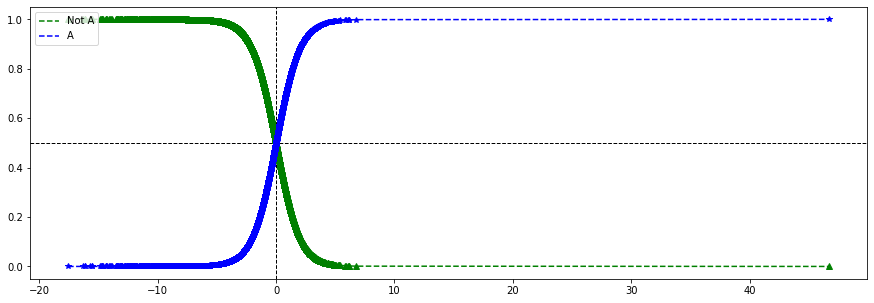

from sklearn.metrics import confusion_matrix, accuracy_score, precision_score, recall_score, f1_score
## 분류 모델의 성능평가
pred=logR.predict(test_x)

test_cm=confusion_matrix(test_y, pred)
test_acc=accuracy_score(test_y, pred)
test_prc=precision_score(test_y, pred)
test_rcll=recall_score(test_y, pred)
test_f1=f1_score(test_y, pred)

print(test_cm)
print('\n')
print('정확도\t{}%'.format(round(test_acc*100,2)))
print('정밀도\t{}%'.format(round(test_prc*100,2)))
print('재현율\t{}%'.format(round(test_rcll*100,2)))
print('F1\t{}%'.format(round(test_f1*100,2)))

[[2768 246][ 349 655]]

정확도 85.19%
정밀도 72.7%
재현율 65.24%
F1 68.77%

소프트맥스 회귀

• 2개 이상의 클래스인 다중 클래스를 지원하도록 일반화 가능
• 이 과정을 다중로지스틱 회귀, 소프트맥스 회귀라 한다.

body = pd.read_csv('./data/bodyPerformance.csv')
# gender 변수 전처리
body['gender']=np.where(body['gender']=='M', 0, 1)
# class 변수 전처리
mapping={'A':0, 'B':1, 'C':2, 'D':3}
body['class_2']=body['class'].map(mapping)

body

from sklearn.model_selection import train_test_split

feature_columns = list(body.columns.difference(['class', 'class_2']))
x=body[feature_columns]
y=body['class_2']

train_x, test_x, train_y, test_y = train_test_split(x,y,stratify=y, train_size=0.7, random_state=1)

print(train_x.shape, test_x.shape, train_y.shape, test_y.shape)

(9375, 11) (4018, 11) (9375,) (4018,)

from sklearn.linear_model import LogisticRegression
## multi_class 클래스의 타입을 지정 ovr는 바이너리, multinomial은 다중 클래스 기본값은 auto
## solver 최적화 문제를 푸는 해를 구할 때 사용할 알고리즘 지정
## C 정규화 강도의 역수
softm=LogisticRegression(multi_class='multinomial', solver='lbfgs', C=10)
softm.fit(train_x, train_y)

from sklearn.metrics import confusion_matrix, accuracy_score

pred=softm.predict(test_x)

test_cm=confusion_matrix(test_y, pred)
test_acc=accuracy_score(test_y, pred)

print(test_cm)
print('\n')
print('정확도\t{}%'.format(round(test_acc*100,2)))

[[707 261 36 0][269 403 300 32]
[ 92 207 525 181][ 13 63 157 772]]

정확도 59.91%