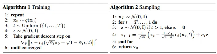
[논문리뷰] Denoising Diffusion Probabilistic Models (DDPM, 2020)

김민서·2024년 7월 7일
0

Diffusion Models

목록 보기
3/8

0. Abstract

1. Introduction

  • 기존 generative models
    - GANs, autoregressive, flow-based, VAE

  • DPM

    • = a parameterized Markov chain

    • 아직까지는 high quality samples에 적용하기는 어렵다

  • Contributions

    • Diffusion models가 high quality samples도 만들 수 있다는 것을 보임
    • certain parameterization에서 denoising score matching과 같다는 것을 보임
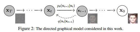
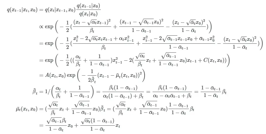
2. Background

  • DPM의 내용인데 notation이 조금 다르다
    • latent variable models of the form pθ(x0):=pθ(x0:T) dx1:Tp_{\theta}(\mathrm{x}_{0}) := \int p_{\theta}(\mathrm{x}_{0:T})\ d\mathrm{x}_{1:T}
    • where x1,...,xT\mathrm{x}_{1},...,\mathrm{x}_{T} are latents of the same dimensionality as the data x0  q(x0)\mathrm{x}_{0}\ \sim \ q(\mathrm{x}_{0})
  • reverse process
    • joint distribution pθ(x0:T)p_{\theta}(\mathrm{x}_{0:T}) := reverse process
    • p(xT)=N(xT;0,I)p(\mathrm{x}_{T})=\mathcal{N}(\mathrm{x}_{T};0,I) 에서 시작하는 Markov chain (with learned Gaussian)으로 정의된다
pθ(x0:T):=p(xT) Πt=1T pθ(xt1xt),where   pθ(xt1xt):=N(xt1;μθ(xt,t),Σθ(xt,t))\begin{aligned} &p_{\theta}(\mathrm{x}_{0:T}):=p(\mathrm{x}_{T})\ \Pi_{t=1}^{T}\ p_{\theta}(\mathrm{x}_{t-1}|\mathrm{x}_{t}),\\ &\mathrm{where}\ \ \ p_{\theta}(\mathrm{x}_{t-1}|\mathrm{x}_{t}):= \mathcal{N}( \mathrm{x}_{t-1};\mu_{\theta}(\mathrm{x}_{t},t), \Sigma_{\theta}(\mathrm{x}_{t}, t))\\ \end{aligned}
  • forward process
    • 다른 latent variable models와 달리 approximate posterior q(x1:Tx0)q(\mathrm{x}_{1:T}|\mathrm{x}_{0})이 fixed되어 있다
    • q(x1:Tx0)q(\mathrm{x}_{1:T}|\mathrm{x}_{0}) := forward process (or diffusion process)
    • Markov chain that gradually adds Gaussian noise to the data according to a fixed variance schedule β1,...,βT\beta_{1},...,\beta_{T}
q(x1:Tx0):=Πt=1Tq(xtxt1),where   q(xtxt1):=N(xt;1βxt1,βtI)\begin{aligned} &q(\mathrm{x}_{1:T}|\mathrm{x}_{0}):=\Pi_{t=1}^{T}q(\mathrm{x}_{t}|\mathrm{x}_{t-1}),\\ &\mathrm{where}\ \ \ q(\mathrm{x}_{t}|\mathrm{x}_{t-1}):=\mathcal{N}(\mathrm{x}_{t};\sqrt{1-\beta}\mathrm{x}_{t-1},\beta_{t}I) \end{aligned}
  • Loss

    • pθp_{\theta} 모델의 negative log likelihood를 minimize하는 방향으로 학습
    • 이 때 variational bound를 이용
      E[log pθ(x0)]  Eq[logpθ(x0:T)q(x1:Tx0)] = Eq[log p(xT)Σt1log pθ(xt1xt)q(xtxt1)] =:L\mathbb{E}[-\mathrm{log}\ p_{\theta}(\mathrm{x}_{0})]\ \leq\ \mathbb{E}_{q}\left[-\mathrm{log}\frac{p_{\theta}(\mathrm{x}_{0:T})}{q(\mathrm{x}_{1:T}|\mathrm{x}_{0})}\right]\ =\ \mathbb{E}_{q}\left[-\mathrm{log}\ p(\mathrm{x}_{T})-\underset{t\geq 1}{\Sigma}\mathrm{log}\ \frac{p_{\theta}(\mathrm{x}_{t-1}|\mathrm{x}_{t})}{q(\mathrm{x}_{t}|\mathrm{x}_{t-1})}\right]\ =:L
    • Comparison with DPM notations
      • negative log likelihood
        • DDPM : E[log pθ(x0)]\mathbb{E}[-\mathrm{log}\ p_{\theta}(\mathrm{x}_{0})]
        • DPM : L=dx(0)q(x(0)) log p(x(0))-L=-\int d\mathrm{x}^{(0)} q(\mathrm{x}^{(0)})\ \mathrm{log}\ p(\mathrm{x}^{(0)})
      • variational bound
        • DDPM : Eq[log p(xT)Σt1log pθ(xt1xt)q(xtxt1)]\mathbb{E}_{q}[-\mathrm{log}\ p(\mathrm{x}_{T})-\underset{t\geq 1}{\Sigma}\mathrm{log}\ \frac{p_{\theta}(\mathrm{x}_{t-1}|\mathrm{x}_{t})}{q(\mathrm{x}_{t}|\mathrm{x}_{t-1})}]
        • DPM : dx(0...T)q(x(0...T)) log[p(x(T))t=1Tp(x(t1)x(t))q(x(t)x(t1))]\int d\mathrm{x}^{(0...T)} q(\mathrm{x}^{(0...T)})\ \mathrm{log}[p(\mathrm{x}^{(T)})∏_{t=1}^{T} \frac{p(\mathrm{x}^{(t-1)}|\mathrm{x}^{(t)})}{q(\mathrm{x}^{(t)}|\mathrm{x}^{(t-1)})}]
  • one-step forward diffusion

    • sampling xt\mathrm{x}_{t} at an arbitrary timestep tt can be done in closed form
    • Use notation αt:=1βt\alpha_{t}:=1-\beta_{t} and αˉt:=Πs=1tαs\bar{\alpha}_{t}:=\Pi_{s=1}^{t}\alpha_{s}, then
      q(xtx0)=N(xt;αˉ x0, (1αˉt)I)q(\mathrm{x}_{t}|\mathrm{x}_{0})=\mathcal{N}(\mathrm{x}_{t};\sqrt{\bar{\alpha}}\ \mathrm{x}_{0},\ (1-\bar{\alpha}_{t})I)
    • Proof
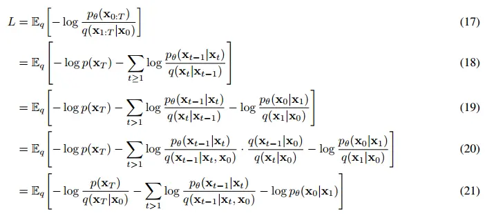
  • Rewrite Loss using KLD

    • DPM의 Appendix B와 같은 내용
    =Eq[DKL(q(xTx0)  p(xT)) + Σt>1DKL(q(xt1xt,x0)  pθ(xt1xt)) + logpθ(x0x1)]=\mathbb{E}_{q}[D_{KL}(q(\mathrm{x}_{T}|\mathrm{x}_{0})\ ||\ p(\mathrm{x}_{T}) )\ +\ \underset{t>1}{\Sigma}D_{KL}(q(\mathrm{x}_{t-1}|\mathrm{x}_{t},\mathrm{x}_{0})\ ||\ p_{\theta}(\mathrm{x}_{t-1}|\mathrm{x}_{t}))\ +\ \mathrm{log}p_{\theta}(\mathrm{x}_{0}|\mathrm{x}_{1})]
    • divided into three parts
      • LT=DKL(q(xTx0)  p(xT))L_{T}=D_{KL}(q(\mathrm{x}_{T}|\mathrm{x}_{0})\ ||\ p(\mathrm{x}_{T}) )
      • Lt1=Σt>1DKL(q(xt1xt,x0)  pθ(xt1xt))L_{t-1}=\underset{t>1}{\Sigma}D_{KL}(q(\mathrm{x}_{t-1}|\mathrm{x}_{t},\mathrm{x}_{0})\ ||\ p_{\theta}(\mathrm{x}_{t-1}|\mathrm{x}_{t}))
      • L0=log pθ(x0x1)L_{0}=\mathrm{log}\ p_{\theta}(\mathrm{x}_{0}|\mathrm{x}_{1})
  • directly compare forward & backward process

    • backward process pθ(xt1xt)p_{\theta}(\mathrm{x}_{t-1}|\mathrm{x}_{t})와 forward posterior(GT) q(xt1xt)q(\mathrm{x}_{t-1}|\mathrm{x}_{t})를 비교
    • q(xt1xt)q(\mathrm{x}_{t-1}|\mathrm{x}_{t})는 계산하기 어렵지만 x0\mathrm{x}_{0} condition이 추가로 주어지면 쉽게 계산할 수 있다
    q(xt1xt,x0)=N(xt1;μ~(xt,x0),β~tI),where   μ~t(xt,x0):=αˉt1βt1αˉtx0+αt(1αˉt1)1αˉtxt   and   β~t:=1αˉt11αˉtβt\begin{aligned} &q(\mathrm{x}_{t-1}|\mathrm{x}_{t},\mathrm{x}_{0})=\mathcal{N}(\mathrm{x}_{t-1};\tilde{\mu}(\mathrm{x}_{t},\mathrm{x}_{0}),\tilde{\beta}_{t}I),\\ &\mathrm{where}\ \ \ \tilde{\mu}_{t}(\mathrm{x}_{t},\mathrm{x}_{0}):=\frac{\sqrt{\bar{\alpha}_{t-1}}\beta_{t}}{1-\bar{\alpha}_{t}}\mathrm{x}_{0}+\frac{\sqrt{\alpha_{t}}(1-\bar{\alpha}_{t-1})}{1-\bar{\alpha}_{t}}\mathrm{x}_{t}\ \ \ \mathrm{and}\ \ \ \tilde{\beta}_{t}:=\frac{1-\bar{\alpha}_{t-1}}{1-\bar{\alpha}_{t}}\beta_{t}\\\end{aligned}
    • Proof

    • 이제 Loss 내의 모든 KLD comparisons는 Gaussian으로만 이루어지게 됨

    • can be calculated in a Rao-Blackwellized fashion with closed form expressions, instead of high variance Monte Carlo estimates

3. Diffusion models and denoising autoencoders

3.1. Forward process and LTL_{T}

  • LT=DKL(q(xTx0)  p(xT))L_{T}=D_{KL}(q(\mathrm{x}_{T}|\mathrm{x}_{0})\ ||\ p(\mathrm{x}_{T}) )
  • βt\beta_{t}를 learnable하게 설정할 수도 있지만 DDPM에서는 fixed schedule로 고정하였음
  • 그러면 posterior q(xTx0)q(\mathrm{x}_{T}|\mathrm{x}_{0})에 learnable parameter가 없으므로 LTL_{T}는 constant

3.2. Reverse process and L1:T1L_{1:T-1}

  • Lt1=Σt>1DKL(q(xt1xt,x0)  pθ(xt1xt))L_{t-1}=\underset{t>1}{\Sigma}D_{KL}(q(\mathrm{x}_{t-1}|\mathrm{x}_{t},\mathrm{x}_{0})\ ||\ p_{\theta}(\mathrm{x}_{t-1}|\mathrm{x}_{t}))

  • pθ(xt1xt)=N(xt1;μθ(xt,t),Σθ(xt,t))  for  1<tTp_{\theta}(\mathrm{x}_{t-1}|\mathrm{x}_{t})=\mathcal{N}(\mathrm{x}_{t-1};\mu_{\theta}(\mathrm{x}_{t},t),\Sigma_{\theta}(\mathrm{x}_{t},t))\ \ \mathrm{for}\ \ 1<t\leq T 에서 μθ,Σθ\mu_{\theta},\Sigma_{\theta}를 어떻게 디자인할까?

  • Σθ(xt,t)\Sigma_{\theta}(\mathrm{x}_{t},t)

    • Σθ(xt,t)=σt2I\Sigma_{\theta}(\mathrm{x}_{t},t)=\sigma_{t}^{2}I 로, sigma는 timestep에 따른 fixed constant로 설정하였음 (X train)
    • σt2\sigma_{t}^{2}β~t:=1αˉt11αˉtβt\tilde{\beta}_{t}:=\frac{1-\bar{\alpha}_{t-1}}{1-\bar{\alpha}_{t}}\beta_{t} 로 놓아도 되지만 (q(xt1xt,x0)q(\mathrm{x}_{t-1}|\mathrm{x}_{t},\mathrm{x}_{0})의 sigma) 실험적으로는 그냥 βt\beta_{t}로 놓는 거랑 별 차이 없었음
    • 따라서 Σθ(xt,t)=βtI\Sigma_{\theta}(\mathrm{x}_{t},t)=\beta_{t} I로 설정
  • μθ(xt,t)\mu_{\theta}(\mathrm{x}_{t},t)

    • Lt1L_{t-1}μ\mu를 이용해서 다시 쓰면,
      Lt1=Eq[12σt2μ~t(xt,x0)μθ(xt,t)2]+CL_{t-1}=\mathbb{E}_{q}\left[\frac{1}{2\sigma_{t}^{2}}||\tilde{\mu}_{t}(\mathrm{x}_{t},\mathrm{x}_{0})-\mu_{\theta}(\mathrm{x}_{t},t)||^{2} \right]+C
    • 여기서 μ~\tilde{\mu}는 forward process posterior mean이고, 우리의 μθ\mu_{\theta} 모델이 이걸 예측하도록 하게 만들면 된다
  • introducing ϵ\epsilon

    • xt(x0,ϵ)=αˉtx0+1αˉtϵ   for   ϵN(0,I)\mathrm{x}_{t}(\mathrm{x}_{0},\epsilon)=\sqrt{\bar{\alpha}_{t}}\mathrm{x}_{0}+\sqrt{1-\bar{\alpha}_{t}}\epsilon \ \ \ \mathrm{for}\ \ \ \epsilon \sim \mathcal{N}(0,I)
      • using one-step diffusion
      • 이걸로 Lt1L_{t-1} 식을 reparameterizing하면 좀 더 단순화시킬 수 있다
      • μ~t\tilde{\mu}_{t} 계산 과정에 넣어보면 증명됨

    Lt1=Ex0,ϵ[12σt2μ~t(xt(x0,ϵ),1αˉtxt(x0,ϵ)1αˉtϵ)μθ(xt(x0,ϵ),t)2]=Ex0,ϵ[12σt21αt(xt(x0,ϵ)βt1αˉtϵ)μθ(xt(x0,ϵ),t)2]\begin{aligned}L_{t-1}&=\mathbb{E}_{\mathrm{x}_{0},\epsilon}\left[\frac{1}{2\sigma_{t}^{2}}\left|\left|\tilde{\mu}_{t}(\mathrm{x}_{t}(\mathrm{x}_{0},\epsilon),\frac{1}{\sqrt{\bar{\alpha}_{t}}}\mathrm{x}_{t}(\mathrm{x}_{0},\epsilon)-\sqrt{1-\bar{\alpha}_{t}}\epsilon)-\mu_{\theta}(\mathrm{x}_{t}(\mathrm{x}_{0},\epsilon),t)\right|\right|^{2} \right]\\ &= \mathbb{E}_{\mathrm{x}_{0},\epsilon}\left[\frac{1}{2\sigma_{t}^{2}}\left|\left|\frac{1}{\sqrt{\alpha_{t}}}\left(\mathrm{x}_{t}(\mathrm{x}_{0},\epsilon) - \frac{\beta_{t}}{\sqrt{1-\bar{\alpha}_{t}}}\epsilon \right)-\mu_{\theta}(\mathrm{x}_{t}(\mathrm{x}_{0},\epsilon),t) \right|\right|^{2}\right]\end{aligned}

    • 이제 μθ\mu_{\theta}1αt(xtβ1αˉtϵ)   given   t\frac{1}{\sqrt{\alpha_{t}}}\left(\mathrm{x}_{t}- \frac{\beta}{\sqrt{1-\bar{\alpha}_{t}}}\epsilon \right)\ \ \ \mathrm{given}\ \ \ t 를 예측해야 함.
      μθ(xt,t)=1αt(xtβt1αˉtϵθ(xt,t))\mu_{\theta}(\mathrm{x}_{t},t)=\frac{1}{\sqrt{\alpha_{t}}}\left(\mathrm{x}_{t}- \frac{\beta_{t}}{\sqrt{1-\bar{\alpha}_{t}}}\epsilon_{\theta}(\mathrm{x}_{t},t) \right)
      • 여기서 ϵθ\epsilon_{\theta}xt\mathrm{x}_{t}의 noise를 예측하는 모델
    • μ\muϵ\epsilon으로 바꿔서 Lt1L_{t-1}을 한번 더 단순화시키면,
      Lt1=Ex0,ϵ[βt22σt2αt(1αˉt)ϵϵθ(αˉtx0+1αˉtϵ,t)2]L_{t-1} = \mathbb{E}_{\mathrm{x}_{0},\epsilon}\left[\frac{\beta_{t}^{2}}{2\sigma_{t}^{2}\alpha_{t}(1-\bar{\alpha}_{t})}\left|\left|\epsilon - \epsilon_{\theta}(\sqrt{\bar{\alpha}_{t}}\mathrm{x}_{0}+\sqrt{1-\bar{\alpha}_{t}}\epsilon, t)\right|\right|^{2} \right]
  • 이제 Lt1L_{t-1}은 denoising score matching과 같은 꼴이 된다

    • Lt1L_{t-1}는 Langevin-like reverse process의 variational bound와 같아짐

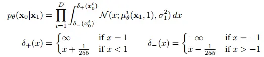
3.3. Data scaling, reverse process decoder, and L0L_{0}

  • 이미지는 {0,1, ..., 255}에서 [-1, 1]로 scaled 되어서 네트워크에 들어간다
  • 마지막 reverse process의 결과는 다시 {0,1, ..., 255} 이미지로 변환되어야 하니까 마지막 pθp_{\theta}는 예외적으로 아래와 같이 정의한다

3.4. Simplified training objective

Lsimple(θ):=Et,x0,ϵ[ϵϵθ(αˉtx0 + 1αˉtϵ,t)2]L_{simple}(\theta):=\mathbb{E}_{t,\mathrm{x}_{0},\epsilon}\left[\left|\left|\epsilon - \epsilon_{\theta}(\sqrt{\bar{\alpha}_{t}}\mathrm{x}_{0}\ +\ \sqrt{1-\bar{\alpha}_t}\epsilon,t) \right|\right|^{2}\right]
  • DDPM의 최종 Loss term
  • tt is uniform between 1 and TT
    • t=1t=1일 때는 3.3.절의 L0L_{0} term을 예외적으로 따른다 (ignore σ12\sigma_{1}^{2} and edge effects)
    • t>1t>1일 때는 3.2.절의 Lt1L_{t-1} term에서 weight를 뺀 것
  • weight를 왜 뺐나?
    • weight βt22σt2αt(1αˉt)\frac{\beta_{t}^{2}}{2\sigma_{t}^{2}\alpha_{t}(1-\bar{\alpha}_{t})}tt가 작아짐에 따라 커진다
    • 따라서 x0\mathrm{x}_{0}에 가까운 매우 작은 noise를 제거하는 단계에 학습이 집중됨
    • 모든 timestep이 동일한 loss 비중을 가지게 하려면 이 weight를 빼는 게 낫다
    • NCSN에서도 timestep에 따른 loss 비중 맞춰주려고 weight를 조작했음

4. Experiments

0개의 댓글