[논문리뷰] Score-based Generative Modeling through Stochastic Differential Equations (Score-SDE, 2021)

김민서·2024년 7월 7일
0

Diffusion Models

목록 보기
4/8

0. Abstract

  • NCSNDDPM을 통합하는 score-SDE framework를 제시
  • 그 외 contributions
    • predictor-corrector framework 제시
    • SDE가 아닌 ODE 버전도 제시해서 sampling efficiency를 높일 수 있도록 함
    • score-SDE를 통해 inverse problem을 해결하는 방법의 뼈대를 제공함

1. Introduction

  • score-based generative model

    • SMLD(==NCSN, Score matching with Langevin dynamics)
    • DDPM
      • sequence of noise corruption을 학습해서 그걸 뒤집어 생성하는 방식
      • continuous state spaces에서 DDPM objective는 score를 implicit하게 계산한다
    • 이 두 방법을 합쳐서 score-based generative model이라 부르기로 한다
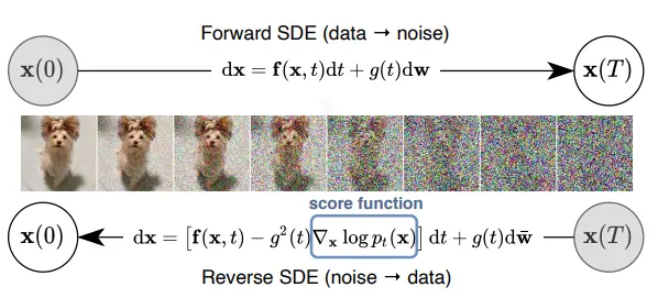
    • 본 논문에서는 SDE(stochastic differential equation)를 이용해서 score-based generative model을 정형화한다
    • finite number of noise X, 여기서는 noise를 continuous하게 씌운다고 생각한다
  • Contributions

    1. Flexible sampling and likelihood computation
      • sampling(reverse process) 시에 어떤 SDE solver든 사용할 수 있다
      • PC (Predictor-Corrector) samplers
        • numerical SDE solvers + score-based MCMC approaches
        • 기존 score-based models에 적용되던 sampling methods를 통합하고 발전시킴
      • deterministic samplers based on probability flow ODE
        • exact likelihood computation
        • allow fast adaptive sampling
        • flexible data manipulation via latent codes
        • uniquely identifiable encoding
    2. Controllable generation
      • training 때는 없었던 conditioning으로 generation을 통제할 수 있음
        • conditional reverse-time SDE는 unconditional score를 이용해서 계산하기 때문
      • 단 하나의 unconditional score model로 class-conditional generation, inpainting, colorization 등 다양한 문제를 풀 수 있다
    3. Unified framework
      • 따로따로였던 SMLD, DDPM 두 방식을 하나의 framework로 통합했다

2. Background

2.1. SMLD

  • Settings
    • pdata(x)p_{data}(\mathrm{x}) : given data distribution
    • pσ(x~x):=N(x~;x,σ2I)p_{\sigma}(\tilde{\mathrm{x}}|\mathrm{x}):=\mathcal{N}(\tilde{\mathrm{x}};\mathrm{x},\sigma^{2}I) : perturbation kernel
    • pσ(x~):=pdata(x)pσ(x~x)dxp_{\sigma}(\tilde{\mathrm{x}}):=\int p_{data}(\mathrm{x})p_{\sigma}(\tilde{\mathrm{x}}|\mathrm{x})d\mathrm{x} : perturbed data distribution
    • noise scheduling σmin=σ1<σ2<...<σN=σmax\sigma_{min}=\sigma_{1}<\sigma_{2}<...<\sigma_{N}=\sigma_{max}
      • σmin\sigma_{min}pσmin(x)pdata(x)p_{\sigma_{min}}(\mathrm{x})\approx p_{data}(\mathrm{x})가 될 만큼 충분히 작아야 하고
      • σmax\sigma_{max}pσmax(x)N(x;0,σmax2I)p_{\sigma_{max}}(\mathrm{x})\approx \mathcal{N}(\mathrm{x};0,\sigma_{max}^{2}I)가 되도록 충분히 커야 함
  • Objective
    θ=argminθ Σi=1Nσi2 Epdata(x) Epσi(x~x)[sθ(x~,σi)x~ log pσi(x~x)22]\theta^{*} =\underset{\theta}{\mathrm{argmin}}\ \Sigma_{i=1}^{N}\sigma_{i}^{2}\ \mathbb{E}_{p_{data}(\mathrm{x})}\ \mathbb{E}_{p_{\sigma_{i}}(\tilde{\mathrm{x}}|\mathrm{x})} \left[||s_{\theta}(\tilde{\mathrm{x}},\sigma_{i})-\nabla_{\tilde{\mathrm{x}}}\ \mathrm{log}\ p_{\sigma_{i}}(\tilde{\mathrm{x}}|\mathrm{x}) ||_{2}^{2}\right]
  • Sampling using Langevin MCMC
    xim=xim1+ϵisθ(xim1,σi)+2ϵizim\mathrm{x}_{i}^{m}=\mathrm{x}_{i}^{m-1}+\epsilon_{i}s_{\theta*}(\mathrm{x}_{i}^{m-1},\sigma_{i})+\sqrt{2\epsilon_{i}}\mathrm{z}_{i}^{m}

2.2. DDPM

  • Settings
    • noise scales 0<β1,β2,...,βN<10<\beta_{1},\beta_{2},...,\beta_N <1 and αi=1βi\alpha_{i}=1-\beta_{i}
    • for each data x0pdata(x)\mathrm{x}_{0}\sim p_{data}(\mathrm{x}), a discrete Markov chain {x0,x1,...,xN}\{\mathrm{x}_{0},\mathrm{x}_{1},...,\mathrm{x}_{N}\} is constructed s.t.
      • p(xixi1)=N(xi;1βixi1,βiI)p(\mathrm{x}_{i}|\mathrm{x}_{i-1})=\mathcal{N}(\mathrm{x}_{i};\sqrt{1-\beta_{i}}\mathrm{x}_{i-1},\beta_{i}I)
    • forward disffusion은 아래와 같이 one-step으로 가능
      • pαiˉ(xix0)=N(xi;αiˉx0,(1αiˉ)I)p_{\bar{\alpha_{i}}}(\mathrm{x}_{i}|\mathrm{x}_{0})=\mathcal{N}(\mathrm{x}_{i};\sqrt{\bar{\alpha_{i}}}\mathrm{x}_{0},(1-\bar{\alpha_{i}})I), where αiˉ=Πj=1iαj\bar{\alpha_{i}}=\Pi_{j=1}^{i} \alpha_{j}
    • SMLD와 비슷한 parameterization으로 살짝 바꿔주기
      • pαi(x~):=pdata(x)pαi(x~x)dxp_{\alpha_{i}}(\tilde{\mathrm{x}}):=\int p_{data}(\mathrm{x})p_{\alpha_{i}}(\tilde{\mathrm{x}}|\mathrm{x})d\mathrm{x} : perturbed data distribution
      • pθ(xi1xi):=N(xi1;11βi(xi+βisθ(xi,i)),βiI)p_{\theta}(\mathrm{x}_{i-1}|\mathrm{x}_{i}):=\mathcal{N}(\mathrm{x}_{i-1};\frac{1}{\sqrt{1-\beta_{i}}}(\mathrm{x}_{i}+\beta_{i}s_{\theta}(\mathrm{x}_{i},i)),\beta_{i}I) : variational Markov chain (reverse)
  • Objective
    • re-weighted variant of ELBO(evidence lower bound)를 이용한 loss
    • DDPM의 LsimpleL_{simple}을 다시 쓴 것
      θ=argminθ Σi=1N(1αi)Epdata(x) Epαi(x~x)[sθ(x~,i)x~log pαi(x~x)22]\theta^{*}=\underset{\theta}{\mathrm{argmin}}\ \Sigma_{i=1}^{N}(1-\alpha_{i})\mathbb{E}_{p_{data}(\mathrm{x})}\ \mathbb{E}_{p_{\alpha_{i}}(\tilde{\mathrm{x}}|\mathrm{x})}[||s_{\theta}(\tilde{\mathrm{x}},i)-\nabla_{\tilde{\mathrm{x}}}\mathrm{log}\ p_{\alpha_{i}}(\tilde{\mathrm{x}}|\mathrm{x}) ||_{2}^{2}]
  • Sampling using reverse Markov chain
    xi1=11βi(xi+βisθ(xi,i))+βizi,   i=N,N1,...,1\mathrm{x}_{i-1}=\frac{1}{\sqrt{1-\beta_{i}}}(\mathrm{x}_{i}+\beta_{i}s_{\theta*}(\mathrm{x}_{i},i))+\sqrt{\beta_{i}}\mathrm{z}_{i},\ \ \ i=N,N-1,...,1

3. Score-based Generative Modeling with SDEs

3.1. Perturbing data with SDEs

  • settings

    • x(0)p0\mathrm{x}(0)\sim p_{0} (data distribution)
    • x(T)pT\mathrm{x}(T)\sim p_{T} (prior distribution)
    • goal : continuous time variable t[0,T]t\in [0,T]에 대해 diffusion process {x(t)}t=0T\{\mathrm{x}(t)\}_{t=0}^{T}를 만드는 것
    • this process can be modeled as the solution to an Ito SDE:
      Forward SDE:   dx=f(x,t)dt+g(t)dw\begin{aligned}\mathrm{Forward\ SDE}:\ \ \ d\mathrm{x}=\mathrm{f} (\mathrm{x},t)dt+g(t)d\mathrm{w}\end{aligned}
      • w\mathrm{w} : standard Wiener process (a.k.a. Brownian motion)
      • f(,t) : RdRd\mathrm{f}(\cdot ,t)\ :\ \mathbb{R}^{d}\rightarrow \mathbb{R}^{d} <= vector valued function called the drift coefficient of x(t)\mathrm{x}(t)
      • g() : RRg(\cdot)\ :\ \mathbb{R}\rightarrow \mathbb{R} <= scalar function called the diffusion coefficient of x(t)\mathrm{x}(t)
        • x(t)\mathrm{x}(t)에 dependent하고 vector valued function인 G(,t)\mathrm{G}(\cdot ,t)로 일반화할 수 있다 (Appendix A)
    • 본 논문에서는 timestep s,ts,t (0s<tT0\leq s<t\leq T)에 대해, x(s)\mathrm{x}(s)에서 x(t)\mathrm{x}(t)로 가는 transition kernel을 pst(x(t)x(s))p_{st}(\mathrm{x}(t)|\mathrm{x}(s))로 표기한다

3.2. Generating samples by reversing the SDE

  • 선행 연구(Anderson, 1982)에 따르면 diffusion process의 reverse도 같은 형태의 diffusion process로 표현된다
    Reverse SDE:   dx=[f(x,t)g(t)2x log pt(x)]dt+g(t)dwˉ\mathrm{Reverse\ SDE}:\ \ \ d\mathrm{x}=[\mathrm{f}(\mathrm{x},t)-g(t)^{2}\nabla_{\mathrm{x}}\ \mathrm{log}\ p_{t}(\mathrm{x})]dt+g(t)d\bar{\mathrm{w}}
    • wˉ\bar{\mathrm{w}} : timeflow가 반대인 (T0T\rightarrow 0) Wiener process
    • dtdt : infinitesimal negative timestep
  • x log pt(x)\nabla_{\mathrm{x}}\ \mathrm{log}\ p_{t}(\mathrm{x}), score of each marginal distribution을 구하면 reverse SDE를 따라 샘플링할 수 있다

3.3. Estimating scores for the SDE

  • 그러면 score x log pt(x)\nabla_{\mathrm{x}}\ \mathrm{log}\ p_{t}(\mathrm{x})를 어떻게 구할까?
  • train a time-dependent score-based model sθ(x,t)\mathrm{s}_{\mathrm{\theta}}(\mathrm{x},t)
  • Score-SDE Objective
    θ=argminθ Et [λ(t)Ex(0)Ex(t)x(0) [ sθ(x(t) , t)x(t) log p0t (x(t)  x(0))22 ] ]\mathrm{\theta^{*}}=\underset{\theta}{\mathrm{argmin}}\ \mathbb{E}_{t}\ \big[\lambda(t)\mathbb{E}_{\mathrm{x}(0)}\mathbb{E}_{\mathrm{x}(t)|\mathrm{x}(0)}\ [\ ||s_{\theta}(\mathrm{x}(t)\ ,\ t)-\nabla_{\mathrm{x}(t)}\ \mathrm{log}\ p_{0t}\ (\mathrm{x}(t)\ |\ \mathrm{x}(0)) ||_{2}^{2}\ ]\ \big]
    • λ : [0,T]R+\lambda\ :\ [0,T]\rightarrow \mathbb{R}^{+}, positive weighting function
      • SMLD, DDPM에서 공통적으로 그랬던 것처럼, 모든 timestep에 대해 비슷한 loss 비중을 가지도록 세팅
      • λ1/E[x(t) log p0t (x(t)  x(0))22]\lambda \propto 1/\mathbb{E}[||\nabla_{\mathrm{x}(t)}\ \mathrm{log}\ p_{0t}\ (\mathrm{x}(t)\ |\ \mathrm{x}(0))||_{2}^{2}]
    • tt is uniformly sampled over [0,T][0,T]
    • x(0)p0(x)\mathrm{x}(0)\sim p_{0}(\mathrm{x}) and x(t)p0t(x(t)x(0))\mathrm{x}(t)\sim p_{0t}(\mathrm{x}(t)|\mathrm{x}(0))
    • 충분한 데이터와 model capacity가 주어졌을 때 sθ(x,t)xlog pt(x)s_{\theta*}(\mathrm{x},t)\approx \nabla_{\mathrm{x}}\mathrm{log}\ p_{t}(\mathrm{x})
    • 여기선 denoising score matching 기준으로 objective를 설정했지만 다른 score matching 기법들을 쓸 수도 있음
  • transition kernel p0t(x(t)x(0))p_{0t}(\mathrm{x}(t)|\mathrm{x}(0))
    • drift coefficient f(,t)\mathrm{f}(\cdot,t)가 affine transform이면 transition kernel은 항상 Gaussian이고, mean과 variance를 closed form으로 구할 수 있다
    • DDPM의 one-step forward diffusion과 같은 것

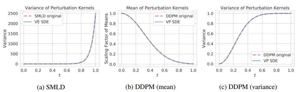
3.4. Examples: VE, VP SDEs and beyond

  • NCSN과 DDPM은 이 score-SDE의 discretization으로 볼 수 있다

    • drift & diffusion coefficient f(,t)\mathrm{f}(\cdot,t) and g(t)g(t) 세팅이 다름
    • 자세한 유도 과정은 Appendix B에
  • NCSN as VE SDE

    • Markov chain : xi=xi1+σi2σi12zi1,   i=1,...,N\mathrm{x}_{i}=\mathrm{x}_{i-1}+\sqrt{\sigma_{i}^{2}-\sigma_{i-1}^{2}}\mathrm{z}_{i-1},\ \ \ i=1,...,N
    • 여기서 NN을 무한으로 보내서 continuous form으로 만들면
      • {σi}i=1N\{\sigma_{i}\}_{i=1}^{N} becomes σ(t)\sigma(t)
      • zi\mathrm{z}_{i} becomes z(t)\mathrm{z}(t)
      • Markov chain {xi}i=1N\{\mathrm{x}_{i}\}_{i=1}^{N} becomes continuous stochastic process {x(t)}t=01, t[0,1]\{\mathrm{x}(t)\}_{t=0}^{1},\ t\in [0,1]
    • 정리하면, NCSN에 해당하는 forward SDE는
      dx=0dt+d[σ2(t)]dtdwd\mathrm{x}=0\cdot dt+\sqrt{\frac{d[\sigma^{2}(t)]}{dt}}d\mathrm{w}
      • tt\rightarrow \infty로 갈 때 variance가 발산하기 때문에 Variance Exploding SDE
  • DDPM as VP SDE

    • Markov chain : xi=1βixi1+βizi1,   i=1,...,N\mathrm{x}_{i}=\sqrt{1-\beta_{i}} \mathrm{x}_{i-1}+\sqrt{\beta_{i}}\mathrm{z}_{i-1},\ \ \ i=1,...,N
    • 마찬가지로 NN을 무한으로 보내고 forward SDE form으로 정리하면
      dx=12β(t)x dt+β(t)dwd\mathrm{x}=-\frac{1}{2}\beta(t)\mathrm{x}\ dt+\sqrt{\beta(t)}d\mathrm{w}
      • tt\rightarrow \infty로 갈 때 variance가 유지되기 때문에 Variance Preserving SDE
  • sub-VP SDE

    • new type of SDEs which perform particularly well on likelihoods
      dx=12β(t)x dt+β(t)(1e20tβ(s)ds)dwd\mathrm{x}=-\frac{1}{2}\beta(t)\mathrm{x}\ dt+\sqrt{\beta(t)(1-e^{-2\int_{0}^{t}\beta(s)ds})}d\mathrm{w}

4. Solving the Reverse SDE

4.1. General-purpose numerical SDE solvers

  • SDE를 푸는 데 이용되는 기존 solvers
    • Euler-Maruyama, stochastic Runge-Kutta methods, etc.
    • reverse SDE를 각기 다르게 discretize해서 stepwise sampling
  • ancestral sampling (of DDPM)
    • recap : xi1=11βi(xi+βisθ(xi,i))+βizi,   i=N,N1,...,1\mathrm{x}_{i-1}=\frac{1}{\sqrt{1-\beta_{i}}}(\mathrm{x}_{i}+\beta_{i}s_{\theta*}(\mathrm{x}_{i},i))+\sqrt{\beta_{i}}\mathrm{z}_{i},\ \ \ i=N,N-1,...,1
    • DDPM에서 정의한 Markov chain을 거꾸로 한 것
    • 이것은 reverse-time VP SDE의 많은 discretizations 중 하나라고 볼 수 있음
  • reverse diffusion samplers
    • reverse-time SDE를 discretize한 것
    • derivations
      • recap
        • Forward SDE:   dx=f(x,t)dt+g(t)dw\mathrm{Forward\ SDE}:\ \ \ d\mathrm{x}=\mathrm{f}(\mathrm{x},t)dt+g(t)d\mathrm{w}
        • Reverse SDE:   dx=[f(x,t)g(t)2x log pt(x)]dt+g(t)dwˉ\mathrm{Reverse\ SDE}:\ \ \ d\mathrm{x}=[\mathrm{f}(\mathrm{x},t)-g(t)^{2}\nabla_{\mathrm{x}}\ \mathrm{log}\ p_{t}(\mathrm{x})]dt+g(t)d\bar{\mathrm{w}}
      • 여기서 tt=0~1을 i=0,1,...,N1i=0,1,...,N-1으로 discretize하면
        • Forward SDE:   xi+1=xi+fi(xi)+gizi\mathrm{Forward\ SDE}:\ \ \ \mathrm{x}_{i+1}=\mathrm{x}_{i}+\mathbf{f}_{i}(\mathrm{x}_{i})+\mathbf{g}_{i}\mathrm{z}_{i}
        • Reverse SDE:   xi=xi+1fi+1(xi+1)+gi+12sθ(xi+1,i+1)+gi+1zi+1\mathrm{Reverse\ SDE}:\ \ \ \mathrm{x}_{i}=\mathrm{x}_{i+1}-\mathbf{f}_{i+1}(\mathrm{x}_{i+1})+\mathbf{g}^{2}_{i+1}s_{\theta^{*}}(\mathrm{x}_{i+1},i+1)+\mathbf{g}_{i+1}\mathrm{z}_{i+1}
      • VE-SDE
        • Markov chain : xi=xi1+σi2σi12zi1,   i=1,...,N\mathrm{x}_{i}=\mathrm{x}_{i-1}+\sqrt{\sigma_{i}^{2}-\sigma_{i-1}^{2}}\mathrm{z}_{i-1},\ \ \ i=1,...,N이므로
        • f=1, g=σi2σi12\mathbf{f}=1,\ \mathbf{g}=\sqrt{\sigma^{2}_{i}-\sigma^{2}_{i-1}}, 이걸 discretized SDE에 대입하면
        • xi=xi+1+(σi+12σi2)sθ(xi+1,σi+1)+σi+12σi2z\mathrm{x}_{i}=\mathrm{x}_{i+1}+(\sigma^{2}_{i+1}-\sigma^{2}_{i})s_{\theta^{*}}(\mathrm{x}_{i+1},\sigma_{i+1})+\sqrt{\sigma^{2}_{i+1}-\sigma^{2}_{i}}\mathrm{z}
      • VP-SDE
        • Markov chain : xi=1βixi1+βizi1,   i=1,...,N\mathrm{x}_{i}=\sqrt{1-\beta_{i}} \mathrm{x}_{i-1}+\sqrt{\beta_{i}}\mathrm{z}_{i-1},\ \ \ i=1,...,N이므로
        • f=1βi1, g=βi\mathbf{f}=\sqrt{1-\beta_{i}}-1,\ \mathbf{g}=\sqrt{\beta_{i}}, 이걸 discretized SDE에 대입하면
        • xi=(21βi+1)xi+1+βi+1sθ(xi+1,i+1)+βi+1z\mathrm{x}_{i}=(2-\sqrt{1-\beta_{i+1}})\mathrm{x}_{i+1}+\beta_{i+1}s_{\theta^{*}}(\mathrm{x}_{i+1},i+1)+\sqrt{\beta_{i+1}}\mathrm{z}
  • unifies DDPM framework
    • timesteps가 충분히 커서 각 βi\beta_{i}가 0에 가깝다면, DDPM의 ancestral sampling과 VP-SDE reverse diffusion sampler는 동일한 식이 된다
    • proof in Appendix E

4.2. PC samplers

  • DDPM ancestral sampling이나 reverse diffusion samplers는 reverse SDE의 해를 이용해서 샘플링하는 과정으로 볼 수 있다

  • NCSN에서는 score-based MCMC approach(annealed Langevin dynamics)를 이용해서 샘플링했는데, 이것은 estimated score function을 따라가도록 설계된 함수

    • 일반적인 SDE와 달리 solution을 improve하기 위한 additional information(score)이 주어진 상황으로 생각할 수 있다
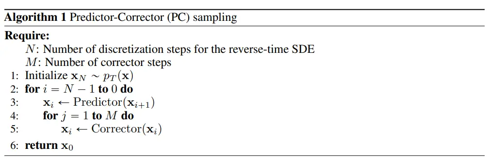
  • Predictor-Corrector (PC) samplers
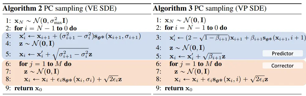
    • predictor

      • next timestep의 sample을 "predict"
      • reverse SDE의 solution
      • 본 논문에서 제안한 reverse diffusion sampler를 써도 되고, Euler-Maruyama같은 기존의 SDE solver 아무거나 가져와서 써도 됨
    • corrector

      • estimated sample의 marginal distribution (score-based)을 참고해서 reasonable한 확률공간에 존재하도록 sample을 "correct"
      • score-based MCMC approach
      • 본 논문에서는 annealed Langevin dynamics를 사용하지만 다른 MCMC methods를 써도 됨
    • 기존의 NCSN은 corrector-only, DDPM은 predictor-only sampling

    • 이제 NCSN, DDPM의 loss 뿐만 아니라 sampling method도 한 framework로 통합했다

  • Experiments

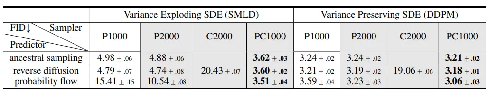
    • CIFAR-10으로 실험, FID로 평가

    • results

      • ancestral sampling보다 reverse diffusion이 약간 나았다
      • corrector only는 성능이 매우 나빴다
      • Predictor only로 timestep을 2배 늘리는 것보다 PC sampling을 이용하는 게 성능이 훨씬 좋았다 (계산량은 같음)
  • Detailed PC sampling algorithms

    • Predictor로는 reverse diffusion sampler, Corrector로는 annealed Langevin Dynamics를 이용함

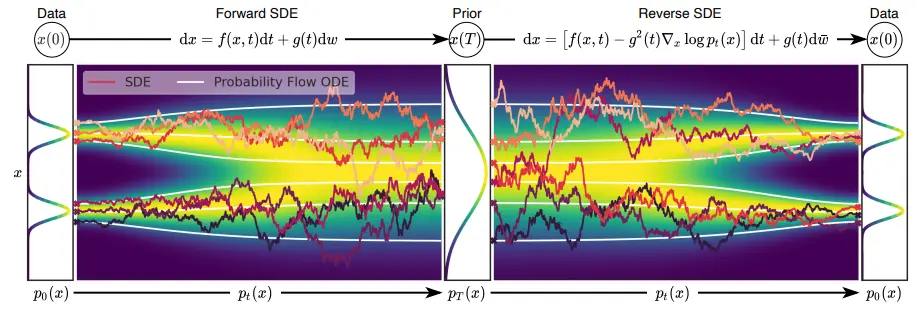
4.3. Probability flow and connection to neural ODEs

  • probability flow ODE
    • For all diffusion processes, there exists a corresponding deterministic process whose trajectories share the same marginal {pt(x)}t=0T\{p_{t}(\mathrm{x})\}_{t=0}^{T} as the SDE
    • 그러한 deterministic process는 아래의 ODE 식을 만족한다
      dx=[f(x,t)12g(t)2x log pt(x)]dtd\mathrm{x}=[\mathrm{f}(\mathrm{x},t)- \frac{1}{2} g(t)^{2}\nabla_{\mathrm{x}}\ \mathrm{log}\ p_{t}(\mathrm{x})]dt
      • derivation at Appendix D.1
      • score를 알고 있으면 deterministic한 trajectory를 얻을 수 있다
      • neural ODE의 한 예시로 볼 수 있다
    • Manipulating latent representations
      • probability flow ODE를 이용하면 x(0)\mathrm{x}(0)를 latent space x(T)\mathrm{x}(T)로 인코딩할 수 있다
      • => we can manipulate latent representation
      • 이 encoding은 기존의 invertible models와는 달리 uniquely identifiable하다
    • Efficient sampling
      • probability flow ODE를 이용해서 샘플링하면 NFE를 줄일 수 있음
        - 실험 결과visual quality를 해치지 않는 선에서 90%까지 줄일 수 있었다
      • accuracy <-> efficiency tradeoff
    • DDIM의 아이디어와 결이 비슷함
    • Consistency Models로 이어짐
  • Exact likelihood computation
    • DDPM loss는 ELBO value를 minimize함
    • neural ODE의 특성을 어떻게 잘 하면 (???) exact likelihood on any input data를 구할 수 있음
    • experiments
      • CIFAR-10으로 실험, bits/dim으로 평가
      • results
        • our DDPM > 기존 DDPM -> exact likelihood를 계산하기 때문
        • DDPM cont. (objective에서 timestep을 continous value로 놓고 학습했을 때)이 discrete version보다 나았음 -> further improves likelihood
        • sub-VP SDE > VP SDE
        • improved architecture (DDPM++) > DDPM

4.4. Architecture improvements

  • 아키텍쳐 좀 손봐서 NCSN++랑 DDPM++ 만들었다
  • guided diffusion 레포에 반영되어 있음

5. Controllable Generation

  • our framework의 continuous한 구조 덕분에 condition y\mathrm{y}를 추가할 수 있다
    • we can also produce samples from p0(x(0)y)p_{0}(\mathrm{x}(0)|\mathrm{y})
  • bayes rule에 의해 x log pt(x  y)=x log pt(x)+x log pt(y  x)\nabla_{\mathrm{x}}\ \mathrm{log}\ p_{t}(\mathrm{x}\ |\ \mathrm{y})= \nabla_{\mathrm{x}}\ \mathrm{log}\ p_{t}(\mathrm{x}) + \nabla_{\mathrm{x}}\ \mathrm{log}\ p_{t}(\mathrm{y}\ |\ \mathrm{x})
  • 이걸 reverse SDE의 기존 score function 자리에 넣으면
    Reverse SDE:   dx=[f(x,t)g(t)2{x log pt(x)+x log pt(y  x)}]dt+g(t)dwˉ\mathrm{Reverse\ SDE}:\ \ \ d\mathrm{x}=[\mathrm{f}(\mathrm{x},t)-g(t)^{2}\{\nabla_{\mathrm{x}}\ \mathrm{log}\ p_{t}(\mathrm{x}) + \nabla_{\mathrm{x}}\ \mathrm{log}\ p_{t}(\mathrm{y}\ |\ \mathrm{x})\}]dt+g(t)d\bar{\mathrm{w}}
    • x log pt(y  x)\nabla_{\mathrm{x}}\ \mathrm{log}\ p_{t}(\mathrm{y}\ |\ \mathrm{x})는 classifier를 따로 학습시켜서 구할 수도 있고 (classifier guidance in ADM), domain knowledge나 heuristics를 이용해서 적당히 정의해도 된다
  • Experiments : class-conditional generation, inpainting, colorization
  • 이 framework를 일반적인 inverse problems에 응용할 수 있다

0개의 댓글