[논문리뷰] Denoising Diffusion Implicit Models (DDIM, 2021)

0. Abstract

• present DDIM
  • DDPM을 non-Markovian process로 generalize
    • generative process가 deterministic해짐
    • 더 빠른 샘플링 가능
  • can produce high quality samples 10~50x faster
    • computation time <-> sample quality tradeoff 있음

1. Introduction

• DDPM requires many iterations

  • DDPM, NCSN과 같은 새로운 iterative generative models는 GAN에 버금가는 성능을 보여줌
  • 얘네는 various levels에서의 Gaussian noise를 예측한 뒤 Markov Chain process를 통해 샘플을 생성한다
  • 이 diffusion process를 수천 번 반복해야 하므로 one-step으로 generation하는 GAN에 비해 굉장히 비효율적임

• DDIM

  • 

  • DDPM과 같은 objective로 학습됨

    • 학습은 DDPM으로 해놓고 샘플링할 때 둘 중에 선택할 수 있음

  • 기존 diffusion process가 Markovian이었던 걸 non-Markovian으로 일반화

  • sampling step 수를 적게 가져갈 때 DDPM보다 나은 성능을 보임

  • “consistency” property를 가짐

    • initial latent variable에 따라 어느정도 결과가 정해져 있음
    • semantically meaningful image interpolation 가능

2. Background

• DDPM의 diffusion process
  $p_{\theta}(x_{0})=\int p_{\theta}(x_{0:T})dx_{1:T},\ \ \ \mathrm{where}\ \ \ p_{\theta}(x_{0:T}):=p_{\theta}(x_{T})\ \Pi_{t=1}^{T}\ p_{\theta}^{(t)}(x_{t-1}|x_{t})$
• parameter $\theta$ 학습은 VLB를 maximize ($p_{\theta}$를 true data distribution $q(x_{0})$에 fit)하는 방향으로 진행
  $\underset{\theta}{\mathrm{max}}\ \mathbb{E}_{q(x_{0})}[\mathrm{log}\ p_{\theta}(x_{0})]\leq \underset{\theta}{\mathrm{max}}\ \mathbb{E}_{q(x_{0},x_{1},…,x_{T})}\ [\mathrm{log}\ p_{\theta}(x_{0:T})-\mathrm{log}\ q(x_{1:T}|x_{0})]$
• forward process
  • fixed inference procedure 이용
  • 여기서 $\alpha$는 DDPM의 $\bar{\alpha}$ ($\alpha$의 cumulative product)와 같음
  • Markov Chain을 Gaussian transition으로 구현했을 때 식은 아래와 같다
    $q(x_{1:T}|x_{0}):=\ \Pi_{t=1}^{T}\ q(x_{t}|x_{t-1}),\ \mathrm{where}\ q(x_{t}|x_{t-1}):=\mathcal{N}\left(\sqrt{\frac{\alpha_{t}}{\alpha_{t-1}}}x_{t-1}, \left(1- \frac{\alpha_{t}}{\alpha_{t-1}} \right)I \right)$
• our latent variable model $p_{\theta}(x_{0:T})$
  • $x_{T}$ to $x_{0}$ sampling을 수행하는 Markov chain
  • reverse process $q(x_{t-1}|x_t)$ (which is intractable)를 approximate
• $\epsilon$-notation
  • DDPM의 one-step diffusion 덕분에 $x_{t}$를 $x_{0}$와 noise의 linear combination으로 바꿔 쓸 수 있다
    $q(x_{t}|x_{0}):=\int q(x_{1:t}|x_{0})dx_{1:(t-1)}=\mathcal{N}(x_{t};\ \sqrt\alpha_{t}x_{0},\ (1-\alpha_{t})I)$
    $x_{t}=\sqrt\alpha_{t} x_{0}+\sqrt{1-\alpha_{t}}\epsilon,\ \ \ \mathrm{where}\ \ \ \epsilon\sim\mathcal{N}(0,I)$
  • $\alpha_{T}$가 0에 충분히 가까우면 $x_{T}$는 true noise에 가까워지므로 $p_{\theta}(x_{T}):=\mathcal{N}(0,I)$로 놓을 수 있다
  • $\epsilon$을 이용해서 training objective를 정리하면 아래와 같음
    $L_{\gamma}(\epsilon_{\theta}):=\Sigma_{t=1}^{T}\gamma_{t}\mathbb{E}_{x_{0}\sim q(x_{0}),\epsilon_{t}\sim \mathcal{N}(0,I)}\ [||\epsilon_{\theta}^{t}(\sqrt\alpha_{t} x_{0}+\sqrt{1-\alpha_{t}}\epsilon_{t})-\epsilon_{t} ||_{2}^{2}]$
  • NCSN의 denoising score matching 기반 loss와도 같다
• Timestep 문제
  • length $T$ of the diffusion process는 DDPM의 성능에 있어서 매우 중요한 hyperparameter임
  • $T$가 클수록 reverse process가 Gaussian에 가까워져서 DDPM의 approximation이 잘 맞는다
  • sampling은 timestep 순서대로 해야 하므로 병렬화가 안 돼서 시간이 오래 걸린다

3. Variational Inference for non-Markovian Forward Processes

3.0. Key Observation

• DDPM objective $L_{\gamma}$를 잘 보면 marginal $q(x_{t}|x_{0})$를 보고 학습하지 joint $q(x_{1:T}|x_{0})$는 상관하지 않는다
• 똑같은 marginal $q(x_{t}|x_{0})$라도 그걸 내놓는 과정 (inference distributions / joints)은 다르게 설계할 수 있다
• -> DDPM objective로 학습시켜놓고, inference할 때는 기존의 Markov process 대신 똑같은 marginal을 내놓는 non-Markovian process를 설계해서 쓸 수 있을 것이다

3.1. non-Markovian Forward Processes

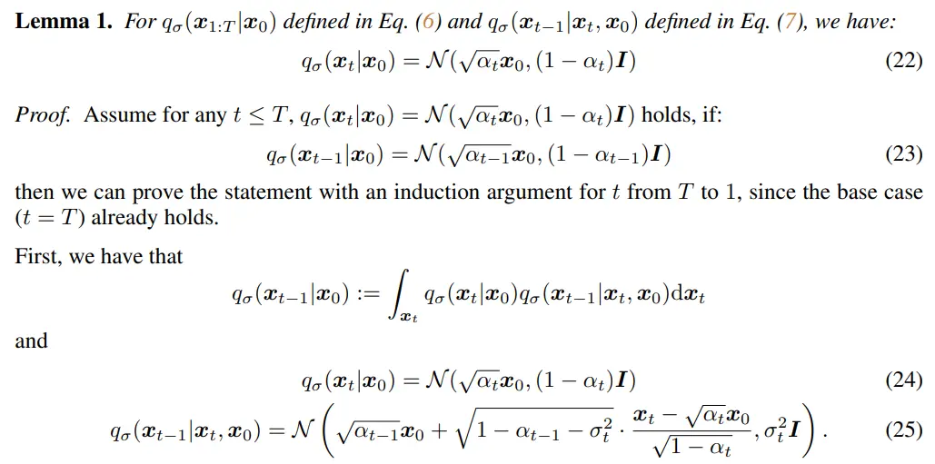
• diffusion kernel들이 $x_{0}$에 dependent하도록 length $T$ real vector $\sigma$에 대한 inference distribution을 새로 정의하자

  $q(x_{1:T}|x_{0}):=\ q_{\sigma}(x_{T}|x_{0})\ \Pi_{t=2}^{T}\ q(x_{t-1}|x_{t},x_{0})$

• DDPM의 objective를 그대로 갖다 쓰려면 marginal $q_{\sigma}(x_{t}|x_{0})=\mathcal{N}(\sqrt{\alpha_{t}}x_{0},(1-\alpha_{t})I)\ \ \mathrm{for\ all\ }t$를 보장해야 함

• 그러면 새로운 diffusion kernel은 아래와 같이 유도됨

  $q_{\sigma}(x_{t-1}|x_{t},x_{0})=\mathcal{N}\left(\sqrt{\alpha_{t-1}}x_{0}+\sqrt{1-\alpha_{t-1}-\sigma_{t}^{2}}\ \cdot\ \frac{x_{t}-\sqrt{\alpha_{t}}x_{0}}{\sqrt{1-\alpha_{t}}},\ \sigma_{t}^{2}I \right)$

  • 귀납법으로 증명 (Appendix B lemma 1)

    • 

    • 

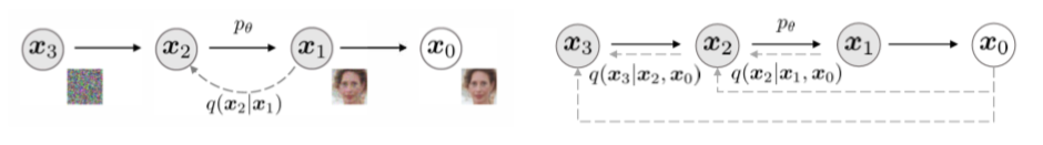
• 이제 Bayes rule을 이용하면 아래와 같이 forward process를 얻을 수 있고, 모든 $x_{t}$는 $x_{t-1}$와 $x_{0}$에 dependent 하게 됨

  $q_{\sigma}(x_{t}|x_{t-1},x_{0})=\frac{q_{\sigma}(x_{t-1}|x_{t},x_{0})\ q_{\sigma}(x_{t}|x_{0})}{q_{\sigma}(x_{t-1}|x_{0})}$
  • forward process는 더 이상 Markovian은 아니지만 여전히 Gaussian이다
  • $\sigma$는 forward process의 stochastic한 정도를 조절하는 변수로 쓰임
    • $\sigma \rightarrow 0$으로 가면 $x_{0},x_{t}$를 알고 있다는 가정 하에 모든 $x_{t-1}$이 fixed된다

3.2. Generative Process and Unified Variational Inference Objective

• generative process

  • $q_{\sigma}(x_{t-1}|x_{t},x_{0})$를 따라하도록 학습된 $p_{\theta}^{(t)}(x_{t-1}|x_{t})$로 generative process $p_{\theta}(x_{0:T})$를 만들었다 치자
  • 샘플링을 하려면 각 단계에서 그 전 단계와 $x_{0}$를 알아야 하는데, 학습할 때와 달리 inference 할 때는 $x_0$를 모른다
    • -> $x_{t}=\sqrt\alpha_{t} x_{0}+\sqrt{1-\alpha_{t}}\epsilon$ 를 이용해서 각 단계마다 $x_{0}$를 예측해서 쓰자
    • denoised observation (prediction of $x_{0}$ given $x_{t}$)
      $f_{\theta}^{(t)}(x_{t}):=(x_{t}-\sqrt{1-\alpha_{t}}\ \cdot\ \epsilon_{\theta}^{(t)}(x_{t}))/\sqrt{\alpha_{t}}$
    • $x_{0}$ 예측을 학습시켜서 좀 더 정교하게 해볼 수도 있지만, 이렇게 단순하게 유도하는 거랑 별로 차이가 없었다
  • 그러면 generative process with fixed prior $p_{\theta}(x_{T})=N(0,I)$는 아래와 같이 쓸 수 있다
    $p_{\theta}^{(t)}(x_{t-1}|x_{t}) = \left\{ \begin{array}{l} \mathcal{N}(f_{\theta}^{(1)}(x_{1}),\sigma_{1}^{2}I)\ \ \ \mathrm{if}\ t=1\\ q_{\sigma}(x_{t-1}|x_{t},f_{\theta}^{(t)}(x_{t}))\ \ \ \mathrm{otherwise} \end{array} \right.$
    • $q_{\sigma}(x_{t-1}|x_{t},x_{0})$을 이용해서 샘플링하되 $x_{0}$는 $f_{\theta}^{(t)}(x_{t})$로 대체한 것

• objective

  • 새로운 objective는 $p_{\theta}(x_{0:T})$와 $q_{\sigma}(x_{1:T}|x_{0})$를 매칭함
    $\begin{aligned}J_{\sigma}(\epsilon_{\theta}) &:= \mathbb{E}_{x_{0:T}\sim q_{\sigma}(x_{0:T})}[\ \mathrm{log}\ q_{\sigma}(x_{1:T}|x_{0})-\mathrm{log}\ p_{\theta}(x_{0:T})] \\ &= \mathbb{E}_{x_{0:T}\sim q_{\sigma}(x_{0:T})} \left[\ \mathrm{log}\ q_{\sigma}(x_T|x_{0}) \ +\ \Sigma_{t=2}^{T}\mathrm{log}\ q_{\sigma}(x_{t-1}|x_{t},x_{0})\ -\ \Sigma_{t=1}^{T}\mathrm{log}\ p_{\theta}^{(t)}(x_{t-1}|x_{t}) - \mathrm{log}\ p_{\theta}(x_{T}) \right] \end{aligned}$

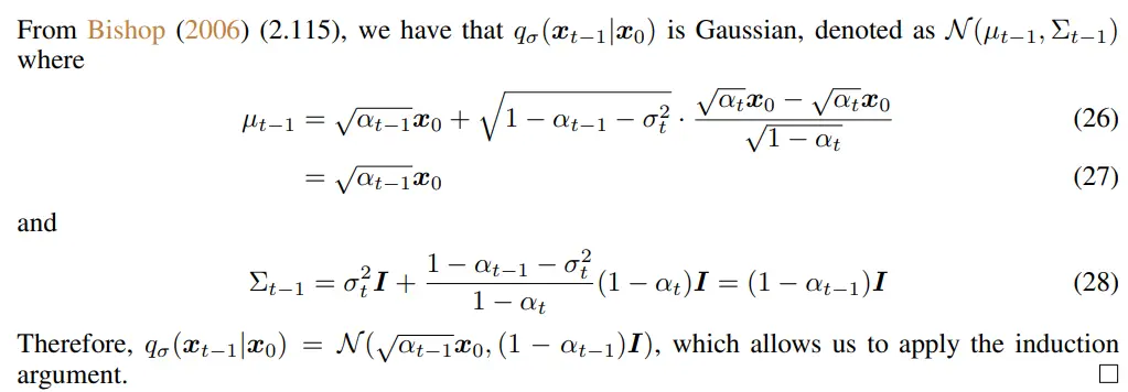
  • 정의에 의하면 $\sigma$ 값에 따라 각기 다른 모델을 train시켜야 하지만, 특정 weight $\gamma$ 조건을 만족하면 $J_{\sigma}$를 DDPM objective $L_{\gamma}$와 같게 만들 수 있다

  • Theorem 1. $For\ all\ \sigma >0,\ there\ exists\ \gamma \in \mathbb{R}_{>0}^{T}\ and\ C\in \mathbb{R},\ s.t.\ J_{\sigma}=L_{\gamma}+C.$

    • Proof (Appendix B)

    • 

    • 31에서 32번 식으로 넘어가는 과정 이해 안 됨 ($d$가 어디서 나온 건지?)

  • $L_{1}$ (DDPM loss) = $J_{\sigma}$

    • 각 timestep에서 예측된 $\epsilon_{\theta}^{(t)}$는 다른 timestep에서는 전혀 쓰이지 않음
    • weight $\gamma$에 따라 timestep 별로 학습되는 속도는 다를 수 있지만, optimal solution에는 영향이 없다
    • 즉, 원래는 $\sigma$마다 $J_{\sigma}=L_{\gamma}+C$를 만족하는 $\gamma$ 값이 다르지만 그걸 모두 $\gamma=1$로 퉁쳐도 어차피 optimal solution은 똑같이 얻어진다
    • 따라서 $\sigma$에 관계 없이 DDPM loss를 그대로 사용해도 된다

4. Sampling from Generalized Generative Processes

4.1. Denoising Diffusion Implicit Models

• diffusion kernel $q_{\sigma}(x_{t-1}|x_{t},x_{0})$의 $x_{0}$자리에 $f_{\theta}^{(t)}(x_{t})$를 대입해서 식을 정리해보면 $x_{t}$로부터 $x_{t-1}$를 샘플링하는 점화식은 아래와 같음
  $x_{t-1}=\sqrt{\alpha_{t-1}}\underbrace{\left(\frac{x_{t}-\sqrt{1-\alpha_{t}}\epsilon_{\theta}^{(t)}(x_{t})}{\sqrt\alpha_{t}}\right)}_{\mathrm{predicted}\ x_{0}}\ +\ \underbrace{\sqrt{1-\alpha_{t-1}-\sigma_{t}^{2}}\ \cdot\ \epsilon_{\theta}^{(t)}(x_{t})}_{\mathrm{direction\ pointing\ to}\ x_{t}} \ +\ \underbrace{\sigma_{t}z}_{\mathrm{random\ noise}}$
• Extreme case 1 : $\sigma_{t}=\sqrt{\frac{1-\alpha_{t-1}}{1-\alpha_{t}}}\sqrt{1-\frac{\alpha_{t}}{\alpha_{t-1}}}$
  • forward process가 Markovian이 됨 (=DDPM)
• Extreme case 2 : $\sigma_{t}=0$
  • forward process becomes deterministic given $x_{t-1}$ and $x_{0}$, except for $t=1$ ($x_{0}$으로 가는 마지막 단계)
  • Theorem 1(DDIM loss = DDPM loss를 증명)에서는 $\sigma>0$인 경우만 생각하므로, 실제로는 $\sigma_{t}\rightarrow 0$으로 근사해야 함

4.2. Accelerated Generation Processes

• 요약: timestep 수를 줄여서 샘플링이 가능하다
• DDPM에서는 generative process $\approx$ reverse process로 두었으므로 forward process가 $T$ steps로 정의되었으면 generative process도 반드시 $T$ steps이어야 했다
• 그러나 objective는 $q(x_{t}|x_{0})$만을 참고하지 forward process가 어떻게 생겨먹었는지와는 관련이 없으므로, generative process $\approx$ reverse process라는 정의만 없으면 timestep 몇 개 빼먹어도 무방하다
• sampling trajectory
  • timestep $[1,...,T]$ 중에 $S$개만 뽑아서 간소화된 forward process $\{x_{\tau_{1}},...,x_{\tau_{S}} \}$를 정의하자
  • 이걸 뒤집어서 ddim sampling을 해도 이론 상으로 문제가 없다
  • sampling trajectory length가 $T$보다 월등히 작으면 샘플링 효율을 크게 높일 수 있음

4.3. Relevance to Neural ODEs

• 요약: $x_{0}$에서 $x_{T}$로 inversion이 가능하다
• DDIM iterate를 ODE 꼴로 바꿔 쓸 수 있다
  • derivation
    • $x_{t}=\sqrt\alpha_{t} x_{0}+\sqrt{1-\alpha_{t}}\epsilon$를 이용하면
      $\frac{x_{t-\Delta t}}{\sqrt{\alpha_{t-\Delta t}}}= \frac{x_{t}}{\sqrt{\alpha_{t}}}+ \left(\sqrt{\frac{1- \alpha_{t-\Delta t}}{\alpha_{t-\Delta t}}} - \sqrt{\frac{1-\alpha_{t}}{\alpha_{t}}} \right) \epsilon_{\theta}^{(t)}(x_{t})$
    • 식을 이쁘게 reparameterization: $\sigma = \frac{\sqrt{1-\alpha}}{\sqrt{\alpha}}$, $\bar{x}= \frac{x}{\sqrt{\alpha}}$
    • initial condition $\sigma (0)=0$으로 설정해서 식을 다시 정리하면
      $d\bar{x}(t) = \epsilon_{\theta}^{(t)}\left(\frac{\bar{x}(t)}{\sqrt{\sigma^{2}+1}} \right) \ d\sigma (t)$
  • 이제 유도된 ODE를 Euler method를 이용해서 풀 수 있다
    • timestep 수가 충분히 많다는 가정 하에 ODE를 풀어서 $x_{0}$로부터 $x_{T}$를 구하는 것이 가능
    • latent encoding이 가능하다 -> 다양한 downstream applications에 쓰일 수 있다
• relevance to "probability flow ODE"
  • DDIM에서 유도된 ODE는 score-SDE에서 정의된 probability flow ODE의 special case라고 볼 수 있다
    • 증명은 Appendix B (proposition 1)에
  • ODE는 같지만 sampling procedure는 좀 다르다
    • $\alpha_{t}$와 $\alpha_{t-\Delta t}$가 충분히 비슷할 때(timestep 수가 많을 때)는 두 procedures가 같지만 fewer timestep으로 샘플링할 때는
    • ODE for VE-SDE(probability flow ODE)는 $dt$에 대한 Euler step을 취하는 반면
    • ODE for DDIM은 $d\sigma (t)$에 대한 Euler step을 취함 (less dependent to $t$)

5. Experiments

• Settings

  • same trained model ($T$=1000)으로 DDPM, DDIM sampling을 모두 수행함
  • $\tau$ (timestep sub-sequences)와 $\sigma$ (stochasticity)에 따른 결과를 관찰함
  • $\sigma_{t}$는 $\sqrt{\frac{1-\alpha_{t-1}}{1-\alpha_{t}}}\sqrt{1-\frac{\alpha_{t}}{\alpha_{t-1}}}$일 때 extreme case(DDPM)이므로 새 변수 $\eta$를 도입해서 parameterization을 좀 더 쉽게 함
    $\sigma_{\tau_{i}}(\eta)=\eta\ \cdot\ \sqrt{\frac{1-\alpha_{\tau_{i-1}}}{1-\alpha_{\tau_{i}}}}\sqrt{1-\frac{\alpha_{\tau_{i}}}{\alpha_{\tau_{i-1}}}}$
    • $\eta=0$일 때 DDIM, $\eta=1$일 때 DDPM
  • $\hat{\sigma}:\ \hat{\sigma_{\tau_{i}}}=\sqrt{1-\frac{\alpha_{\tau_{i}}}{\alpha_{\tau_{i-1}}}}$
    • random noise의 std가 1보다 큰 경우
    • $\eta$로 치면 $\eta>1$인 경우 (DDPM)

• 5.1. Sample Quality and Efficiency

  • 

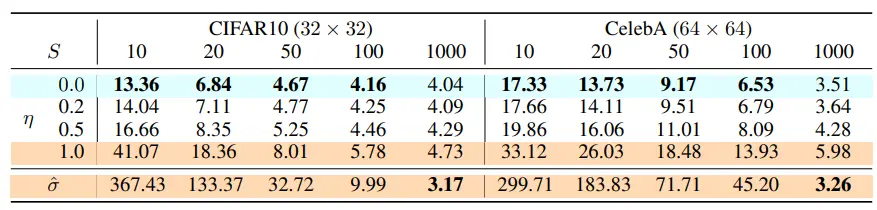
  • CIFAR10, CelebA에서 실험, FID로 평가

  • timestep 수에 따른 sample quality <-> computational cost tradeoff가 있었다

  • 같은 timestep일 때 DDIM이 성능이 더 좋았다

  • 다만 full timestep을 이용한 경우 $\hat{\sigma}$가 가장 좋았음

    • $\hat{\sigma}$ 케이스는 non-Markovian sampling의 정의에서 벗어나기 때문에 timestep을 줄이는 조건이 ill-suited하다

  • DDIM으로 10x ~ 50x speedup이 가능하다

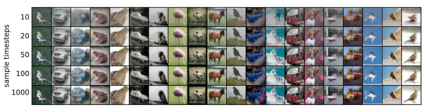
• 5.2. Sample Consistency in DDIMs

  • 

  • DDIM의 경우 generative process가 deterministic하므로, $x_{0}$는 initial state $x_{T}$에 따라 결정된다

  • -> $x_{T}$가 fixed 되어 있으면 timestep을 달리 해도 퀄리티만 살짝 다른 같은 결과물이 나온다

  • $x_{T}$ alone would be an informative latent encoding of the image

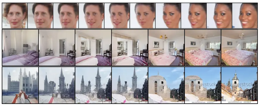
• 5.3. Interpolation in Deterministic Generative Processes

  • 

  • 5.2.에 이어서, 서로 다른 두 $x_{T}$를 섞으면 결과물 $x_{0}$끼리 적당히 interpolation된 결과물이 나온다 (semantically meaningful interpolation)

  • DDIM은 latent variable 단에서 high level contents를 직접 조절할 수 있다 (DDPM에서는 안 됨)

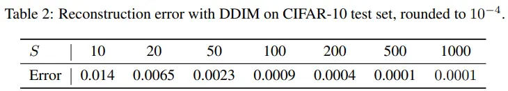
• 5.4. Reconstruction from Latent Space

  • 

  • DDIM은 particular ODE의 Euler integration이므로, $x_{0}$로부터 $x_{T}$를 인코딩한 뒤 다시 $x_{T}$로 $x_{0}$를 복원할 수 있다

  • CIFAR10으로 reconstruction 실험해봤더니 잘 됐다, timestep 수가 많을 수록 error가 적었음

  • DDPM에서는 stochastic nature 때문에 이게 안 된다