0. Abstract
- Diffusion Models이 이전까지 SOTA였던 GAN보다 우수함을 실험적으로 보여줌
- 처음으로 diffusion guidance를 제시함
- 깃헙 guided-diffusion 레포
1. Introduction
- GAN
- image generation tasks에서 SOTA
- FID, Inception Score, Precision
- limitations
- diversity가 떨어짐
- 학습이 불안정함
- 위의 단점들 때문에 확장성이 떨어짐
- image generation tasks에서 SOTA
- GAN vs. Diffusion
- 아직까지는 GAN이 성능이 더 좋음
1) GAN은 오랜 시간 연구되면서 충분히 튜닝되었기 때문. 반면 디퓨젼은 갓 태어난 날것이니까
2) GAN은 diversity <-> fidelity tradeoff에서 fidelity를 선택했기 때문에 퀄리티가 좋은 것
- 아직까지는 GAN이 성능이 더 좋음
- 본 논문에서는 diffusion을 약간 손보면 GAN보다 성능이 좋아짐을 실험적으로 보임
2. Background
- Diffusion Models
- Improved DDPM
- Contributions
- variance 를 상수로 fix하는 것은 optimal이 아니라고 주장
- 기존 DDPM에서는 로 세팅했었다
- propose to parameterize
- recap DDPM
- reverse process 를 학습하려면 forward process 를 뒤집은 forward posterior 와 비교해야 했다
- 그런데 는 구하기 어려우므로 계산이 쉬운 를 대신 썼음
- forward process 로 주어졌고
- forward posterior는
- 로 주어짐
- 따라서 는 각각 reverse process variance의 upper&lower bound에 해당함
- recap DDPM
- 과 를 동시에 학습하기 위해 weighted sum objective 를 도입함
- variance 를 상수로 fix하는 것은 optimal이 아니라고 주장
- sample quality를 떨어뜨리지 않고도 sampling step 수를 줄일 수 있음
- Contributions
- DDIM
- 본 논문에서는 Improved DDPM의 objective & parameterization, DDIM의 sampling strategy를 차용함
- quality metrics로는 FID를 메인으로 사용하였음
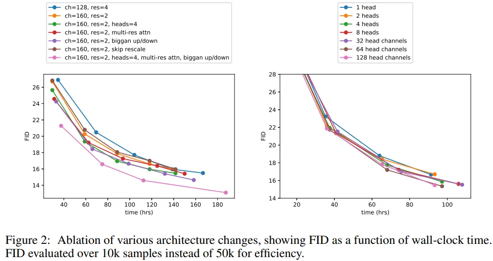
3. Architecture Improvements
-
previous works
-
architectural changes
- Increasing depth vs. width, holding model size relatively constant
- Increasing the number of attention heads
- Using attention at 32x32, 16x16, and 8x8 resolutions rather than only at 16x16
- Using the BigGAN residual block for upsampling & downsampling the activations (from score-SDE)
- Rescaling residual connections with (from [score-SDE], StyleGAN)
-
ImageNet 128x128으로 학습시키고 FID로 성능 평가함
-
Adaptive Group Normalization
- AdaGN이라는 layer로도 실험해 봄
- groupnorm 연산 이후 residual block과 더불어 timestep and class embedding도 함께 활용하기
- adaptive instance norm(AdaIN), FiLM과 유사함
-
- : intermediate activations of the residual block
- : obtained from a linear projection of the timestep & class embedding
- AdaGN이라는 layer로도 실험해 봄
-
Setting default model architectures
- 2 residual blocks per resolution
- multiple heads with 64 channels per head
- attention at 32, 16 and 8 resolutions
- BigGAN residual blocks for up and downsampling
- AdaGN for injecting timestep & class embeddings into residual blocks
4. Classifier Guidance
4.0. How to condition diffusion models?
- 우리는 이미 AdaGN layer에서 class information을 주입하고 있음
- classifier 를 이용해서 diffusion generation을 발전시킬 수 있음
- 편의를 위해 notation에서 일부 는 생략하였음 ()
4.1. Conditional Reverse Noising Process
-
unconditional reverse process 를 label 로 컨디셔닝한 확률은 아래와 같이 나타낼 수 있다.
- : 확률의 합을 1로 만들어주는 normalizing constant
- 본래 이 식은 intractable하지만 DPM에 의해 perturb Gaussian distribution으로 근사될 수 있다
-
-
는 보다 낮은 curvature를 가진다 (???)
- diffusion step 수가 많아질 수록 으로 가기 때문
- 따라서 를 근처에서의 Taylor expansion으로 근사할 수 있다
- 여기서 이고 은 constant이므로
-
conditional transition operator는 unconditional operator와 비슷한 Gaussian으로 근사되지만, mean이 만큼 shift된다
-
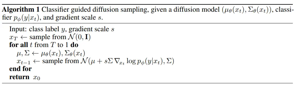
-
diffusion model output 와 classifier gradient를 구한 후, 에 classifier gradient를 더해준다
-
는 scale factor
-
4.2. Conditional Sampling for DDIM
- 4.1.의 알고리즘은 stochastic diffusion sampling에만 적용 가능하고, DDIM 같은 deterministic sampling에는 쓸 수 없다
- score-based conditioning trick 이용하기
- connection between diffusion models and score matching:
- 이제 를 score function을 포함하는 꼴로 변형한 뒤 거기에 diffusion network 를 대입해보자
- 이제 새로운 epsilon prediction 를 아래와 같이 정의한다
- 이게 어떻게 나온건지?? 이해 안 됨
- DDIM같은 샘플러를 이용할 때 기존의 대신 을 쓰면 된다
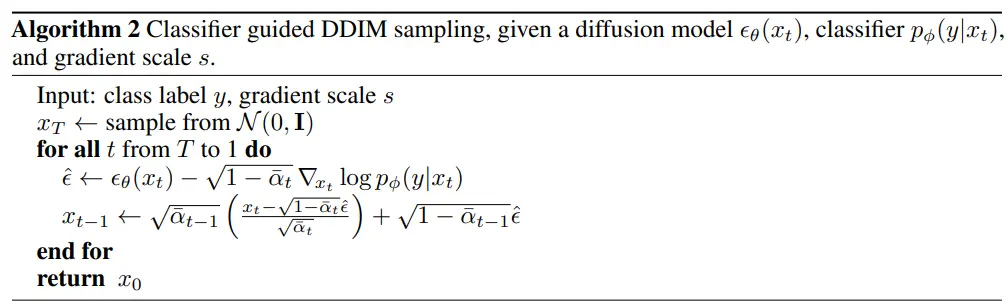
- 이게 어떻게 나온건지?? 이해 안 됨
4.3. Scaling Classifier Gradients
-
Training classifier
- UNet의 downsampling trunk에 attention pool을 붙여서 classifier를 만들었다
- diffusion model 학습할 때 들어가는 input을 classifier에도 input으로 넣어서 학습함
- 학습된 classifier를 classifier guidance에 이용
-
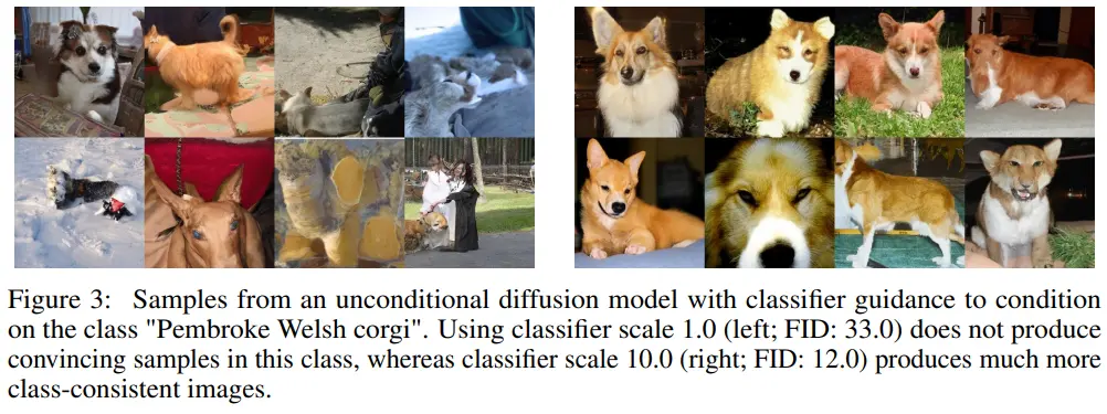
gradient scale
- Figure 4 참고
- 로 놓으면 원하는 클래스의 결과가 잘 안 나왔다
- 정도로 높이면 거의 100% 해당 클래스로 분류되는 결과가 나왔다
- 의 값이 커질수록 classifier gradient의 반영 비율이 exponential하게 높아지기 때문
-
with conditional diffusion model
- Table 4 참고
- 여태까지는 unconditional model 에 대한 classifier guidance만 다뤘음
- conditional diffusion model 에도 똑같은 방식으로 guidance를 줄 수 있다
- unconditional/conditional model 모두 guidance를 줬을 때 결과물이 좋았고, conditional model + guidance 둘 다 썼을 때 가장 좋은 FID를 달성할 수 있었다
-
GAN과의 비교
- Figure 5 참고
- BigGAN-deep과 비교했을 때, classifier guidance가 FID<->IS tradeoff 면에서는 우수하지만 precision<->recall tradeoff 면에서는 GAN보다 약간 뒤쳐졌다