[ML] Support Vector Machine (SVM)

Support Vector Machine

• hyperplane 과 가장 가까운 support vector 사이의 거리 margin을 최대가 되도록 하는 알고리즘

  • hyperplane : class 를 구분짓는 평면. N 차원일 경우 N-1 차원으로 표현되는 평면
  • support vector : hyperplane 과 가장 가까운 sample
  • margin : hyperpiane 과 support vector 사이의 거리

• classfication(분류), regression (회귀) and outliers detection (이상치 탐지) 에 활용된다.

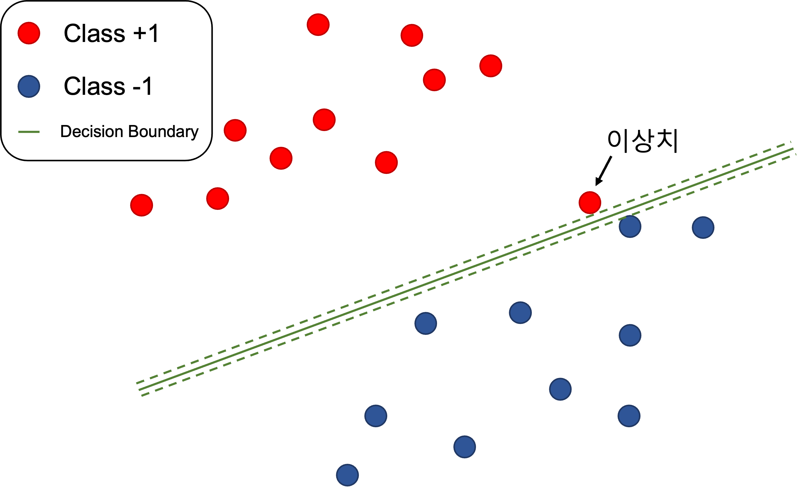
soft margin classification

• 현실에서는 noise, outlier (이상치) 로 선형 분류가 불가능하거나 마진이 작아지는 문제가 생길 수 있다.
  • 이를 보정하기 위해 slack variable ξ 를 허용하여 보다 조건을 완화하고 여유 있게 최적화

kernel trick

• 선형 분류가 불가능한 경우 (non-linearly separable) kernel trick 을 통해 비선형 분류로 활용한다.
  • 보다 고차원으로의 mapping function 을 통해 매핑,
  • hyperplane을 찾을 수 없던 모델에 대해 hyperplane을 찾을 수 있도록 한다
  • 대표적인 커널 함수로 polynomial, gaussian, sigmoid kernel 등이 있다.
  • scikit-learn SVM 라이브러리에서는 linear, polynomial, rbf, sigmoid 옵션으로 제공된다.

>>> linear_svc = svm.SVC(kernel='linear')
>>> linear_svc.kernel
'linear'
>>> rbf_svc = svm.SVC(kernel='rbf')
>>> rbf_svc.kernel
'rbf'

Scikit-learn 으로 SVM training

• SVM training

from sklearn.svm import SVC
from sklearn import datasets
from sklearn.model_selection import train_test_split
from sklearn.preprocessing import StandardScaler
from matplotlib.colors import ListedColormap
import matplotlib.pyplot as plt
import numpy as np


def train_svm():
    """
    iris(붓꽃) 데이터셋으로 꽃받침 길이, 꽃잎 길이 2개 feature 로 분류하기
    :return:
    """
    iris_dataset = datasets.load_iris()
    x = iris_dataset.data[:, [2, 3]] # 꽃 데이터셋 중 일부 feature 만 추출 (꽃받침, 꽃길이)
    y = iris_dataset.target # 꽃 품종 label

    # test_size : test data와 training data 비율. 0.3이면 test 30%, training 70%
    # random_state: 데이터셋을 섞기 위해 사용되는 random seed. 고정일 경우 매번 동일하게 재현
    # stratify : stratification (계층화). training, test 데이터 셋의 label 비율을 input 데이터셋과 동일하게 함
    x_train, x_test, y_train, y_test = train_test_split(x, y, test_size=0.3, random_state=1, stratify=y)

    print(f'class label : {np.unique(y)}')

    # stratification 결과 체크
    print(f'y original data set label count : {np.bincount(y)}')
    print(f'y training data set label count : {np.bincount(y_train)}')
    print(f'y test data set label count : {np.bincount(y_test)}')

    # feature 표준화
    sc = StandardScaler()
    # traing data set 의 feature dimension 마다 평균과 표준 편차 계산
    sc.fit(x_train)

    # transform: 평균과 표준 편차로 data set 을 표준화
    x_train_std = sc.transform(x_train)
    x_test_std = sc.transform(x_test)

    # training
    svm = SVC(kernel='linear', C=1.0, random_state=1)
    svm.fit(x_train_std, y_train)

    # 시각화를 위해 training, test data set 결합
    x_combined_std = np.vstack((x_train_std, x_test_std))
    y_combined = np.hstack((y_train, y_test))

    # 시각화
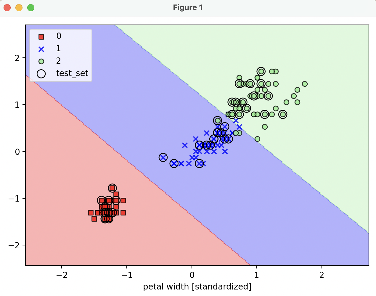
    plot_decision_regions(x=x_combined_std, y=y_combined, classifier=svm, test_idx=range(105,150))
    plt.xlabel('petal length [standardized]')
    plt.xlabel('petal width [standardized]')
    plt.legend(loc='upper left')
    plt.tight_layout()
    plt.show()

• 시각화

def plot_decision_regions(x, y, classifier, test_idx=None, resolution=0.02):
    """
    시각화
    :param x: 붓꽃 데이터셋 feature (0번 열 : 꽃받침 길이, 1번 열 : 꽃잎 길이)
    :param y: class label
    :param classifier: 분류기
    :param test_idx:
    :param resolution:
    :return:
    """
    # 마커, 컬러맵 설정
    markers = ('s', 'x', 'o', '^', 'v')
    colors = ('red', 'blue', 'lightgreen', 'gray', 'cyan')
    cmap = ListedColormap(colors[:len(np.unique(y))])

    # decision boundary (결정 경계) 그리기
    # feature
    x1_min, x1_max = x[:, 0].min() - 1, x[:, 0].max() + 1 # feature column 0 -> 꽃받침 길이
    x2_min, x2_max = x[:, 1].min() - 1, x[:, 1].max() + 1 # feature column 1 ->  꽃잎 길이

    # meshgrid : 축에 해당하는 1차원 배열을 받아 벡터 공간의 모든 좌표를 담은 행렬을 반환
    xx1, xx2 = np.meshgrid(np.arange(x1_min, x1_max, resolution),
                           np.arange(x2_min, x2_max, resolution))
    # ravel : 배열을 1차원 배열로 펼치기
    # T : transpose
    # 2개 배열을 펼치고 각 행으로 붙이고 transpose 하여 2개의 열로 변환, 이후 class label 예측
    z = classifier.predict(np.array([xx1.ravel(), xx2.ravel()]).T)
    # xx1, xx2 와 같은 차원의 그리드로 크기 변경
    z = z.reshape(xx1.shape)
    # contourf : 등고선 그래프 그리기
    plt.contourf(xx1, xx2, z, alpha=0.3, cmap=cmap)
    # x, y축 limit 설정
    plt.xlim(xx1.min(), xx1.max())
    plt.ylim(xx2.min(), xx2.max())

    for idx, cl in enumerate(np.unique(y)):
        plt.scatter(x=x[y == cl, 0], y=x[y == cl, 1],
                    alpha=0.8, c=colors[idx],
                    marker=markers[idx], label=cl,
                    edgecolor='black')

    if test_idx:
        x_test, y_test = x[test_idx, :], y[test_idx]

    plt.scatter(x_test[:, 0], x_test[:, 1],
                facecolors='none', edgecolor='black', alpha=1.0,
                linewidth=1, marker='o',
                s=100, label='test_set')

reference

• 서적 '머신 러닝 교과서 with 파이썬, 사이킷런, 텐서플로 개정 3판'
• scikit-learn SVM Docs
• SVM 이미지 출처
• soft margin SVM 이상치 이미지 출처