1. Measuring Purity

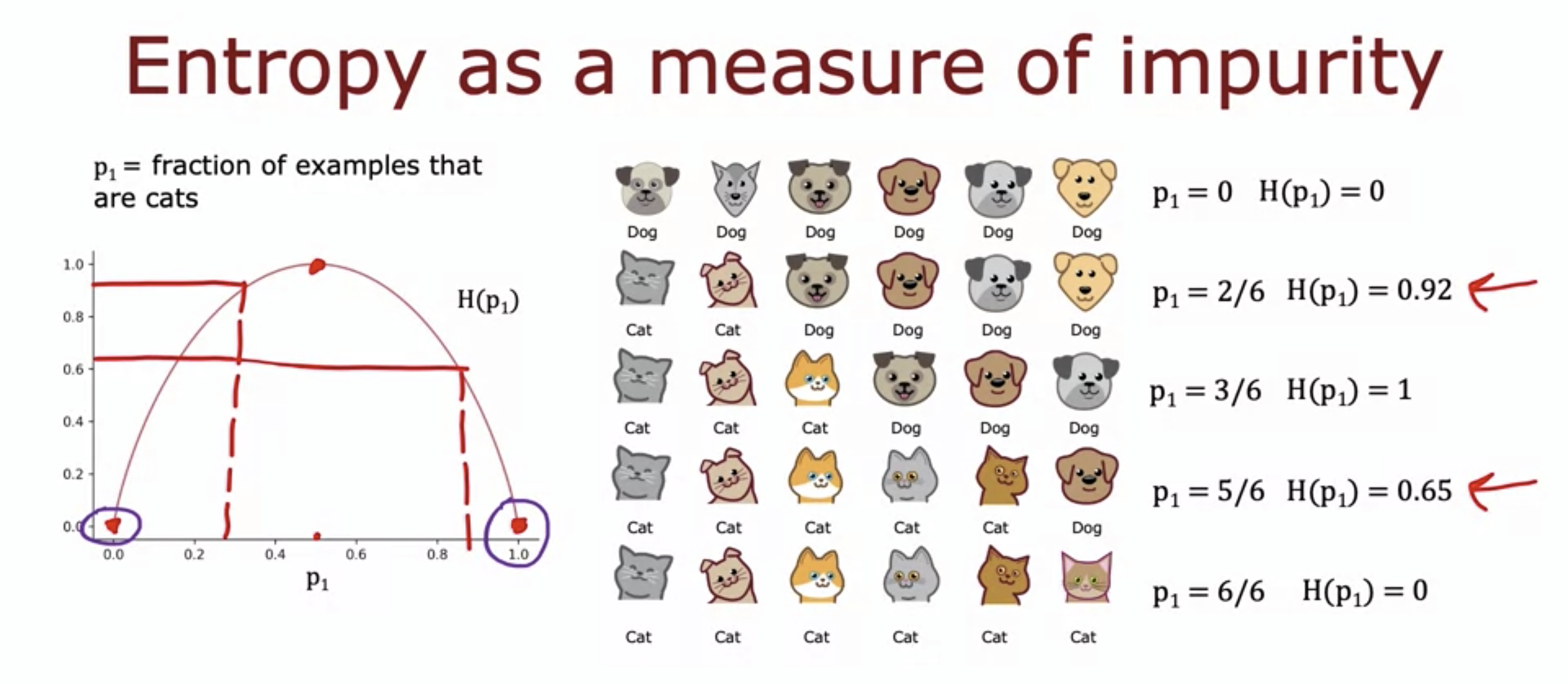
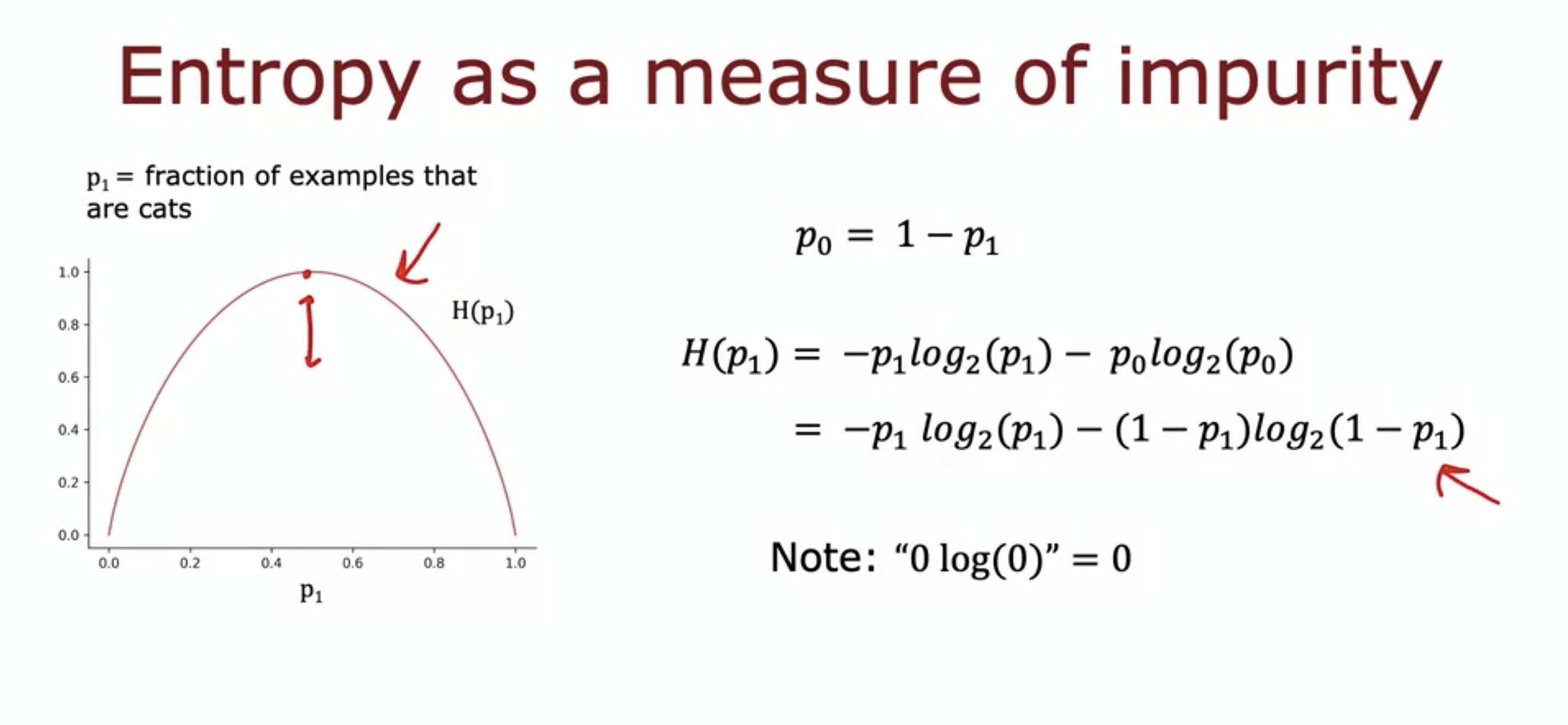
• The entropy function (denoted by H(p1), where p1 is the fraction of examples that are cats in this case) can be a measure of purity in one batch of example.
• If the batch is completely pure, then it is either that the whole batch is dog, or whole batch is cat.

• The entropy function kinda looks like the logistic loss function, and there is a mathematical rationale for it (can search it up later)
• The log base is 2 so that when p = 0.5 the entropy value is 1.
  • If different log base is used, say an e, then the function shifts vertically.

2. Choosing a split: Information Gain

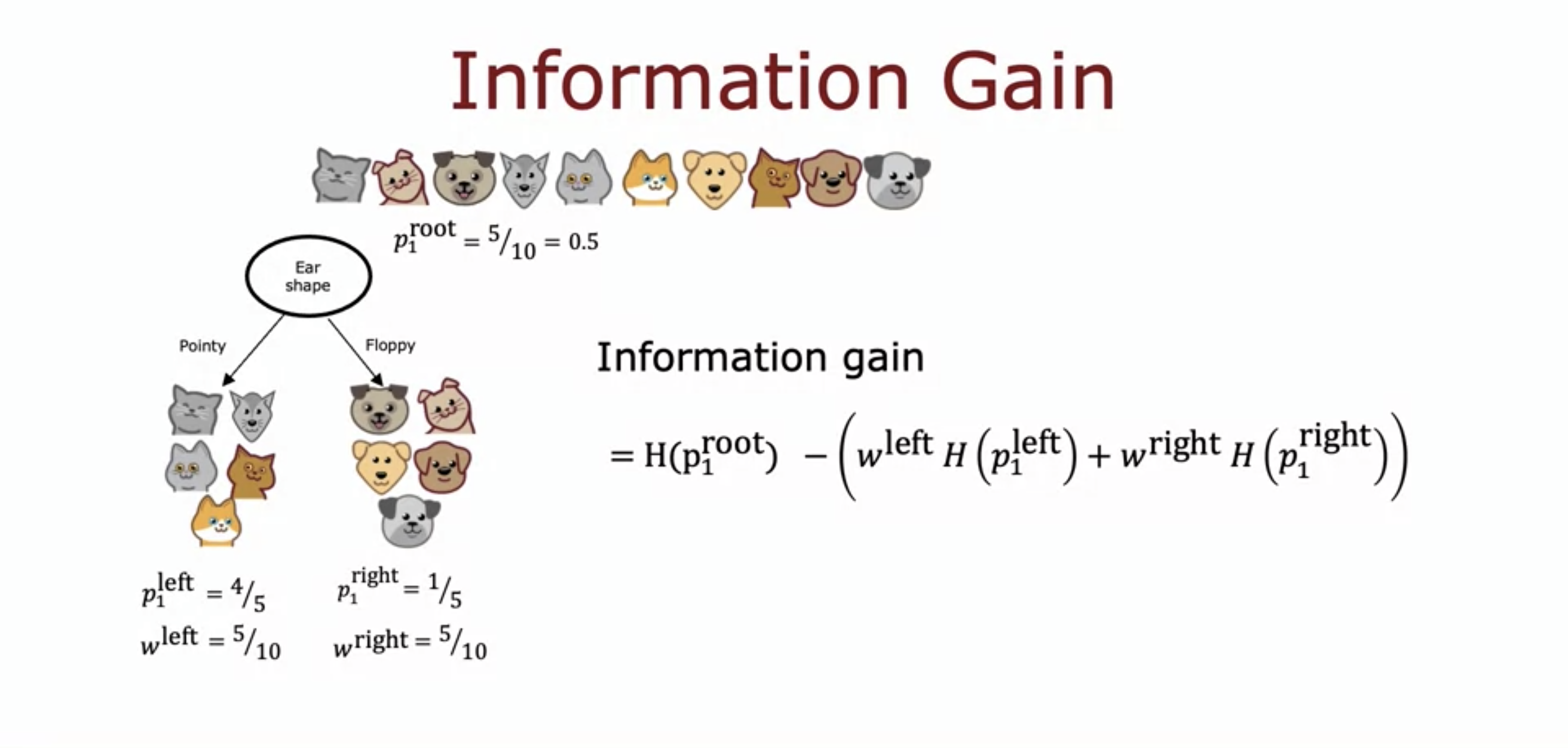
The reduction of impurity is called information gain.

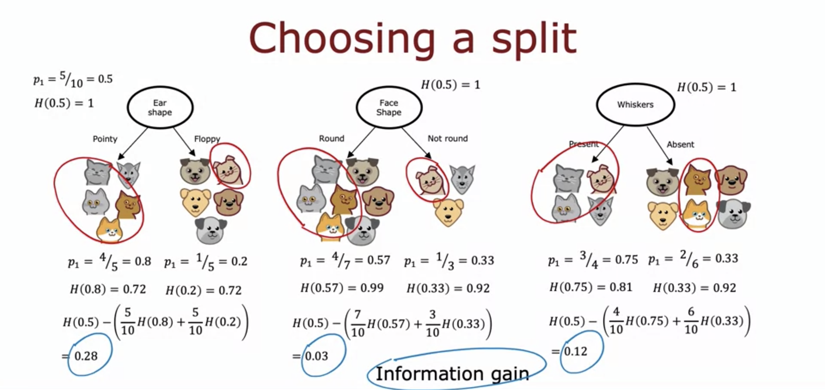
• We first compute the weighted average of the entropy.
  • The reason we compute weighted average instead of just the entropies on the left and the right branch is that the number of the examples on each branch should also be taken into consideration.
  • So we multiply the entropy by the fraction and add them.
• We then subtract the weighted average from the entropy of the previous node .
  • This is to find out how effective the splitting of data set was.
  • The bigger the difference is, the more effective the splitting was, since that means the entropy of the current node is much lower.
• Therefore, from the example of the cats, splitting by the ear shape should be chosen.

• The higher the information gain is, the more pure the data set are after splitting by the node.

3. Putting it together

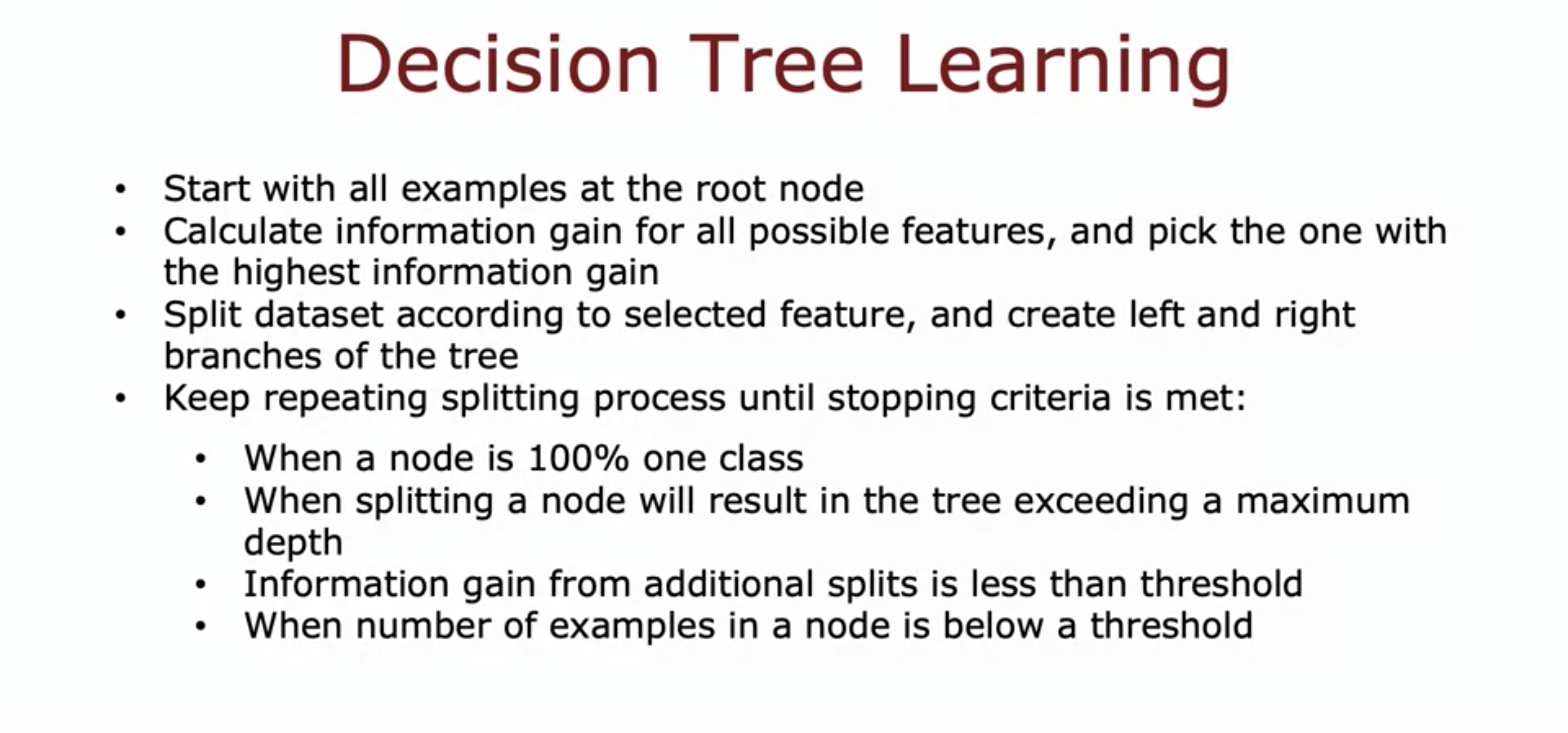
As the slide suggests.

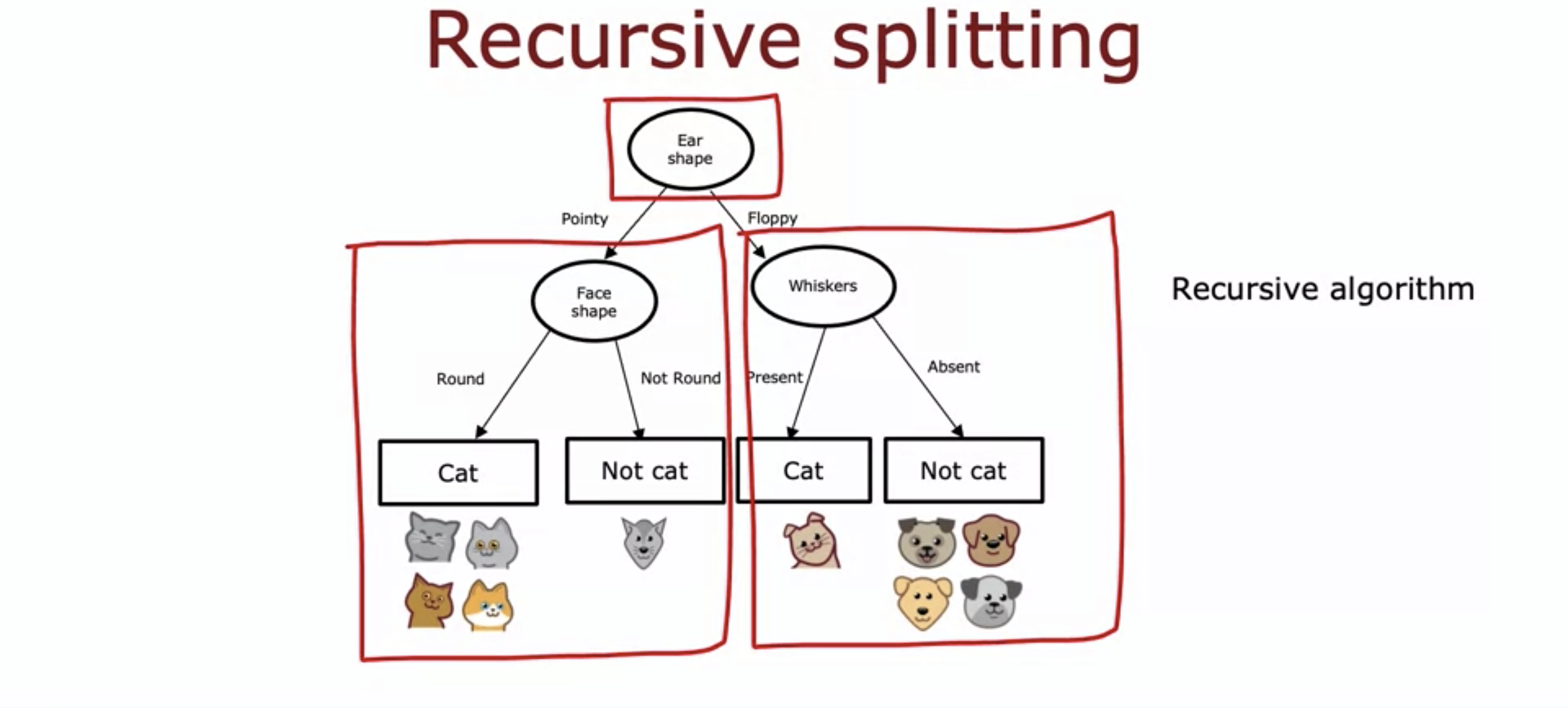
• The process goes like this:
  • Check if the ending condition is met.
    • If yes, then stop.
    • If no, continue.
  • Calculate the information gain, then select a feature to split by.
  • Repeat the process until a subtree is finished, then which other subtrees will continue working until every tree is calculated.
  • This process is known as recursive algorithm.
• There are open source libraries that support this recursive process.
• Libraries also help choosing the maximum depth.
  • The larger the maximum depth, the bigger the tree.
  • The bigger the tree, the riskier it is to overfitting.
  • In theory, we could use the cross-validation set of different maximum depths and calculate the best maximum depth,
  • But there are libraries that help you do that.

4. Using one-hot encoding of categorical variables

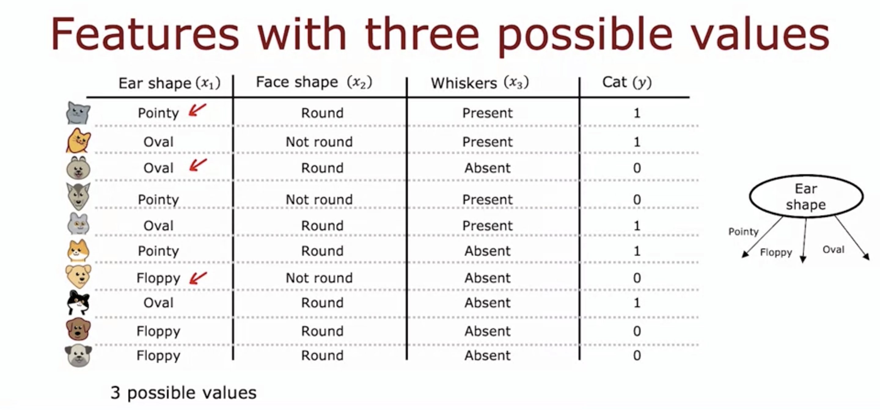
• Instead of just two ear shapes, now we have 3 including oval shape.

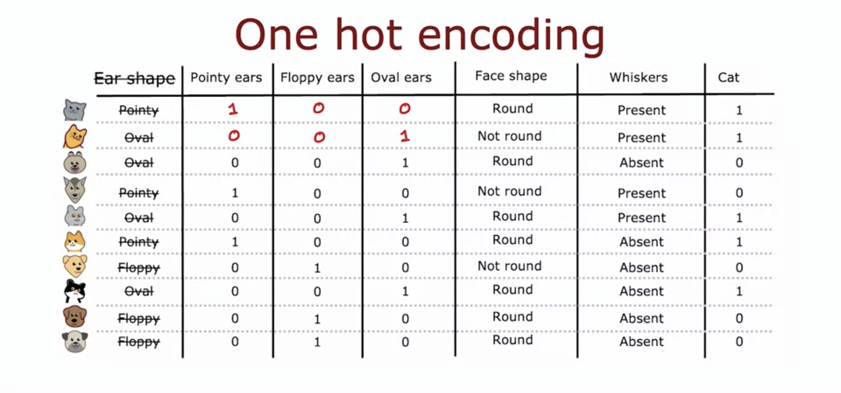
• Only one of the 3 types of ear shapes has the value 1.
• This is known as one hot encoding.

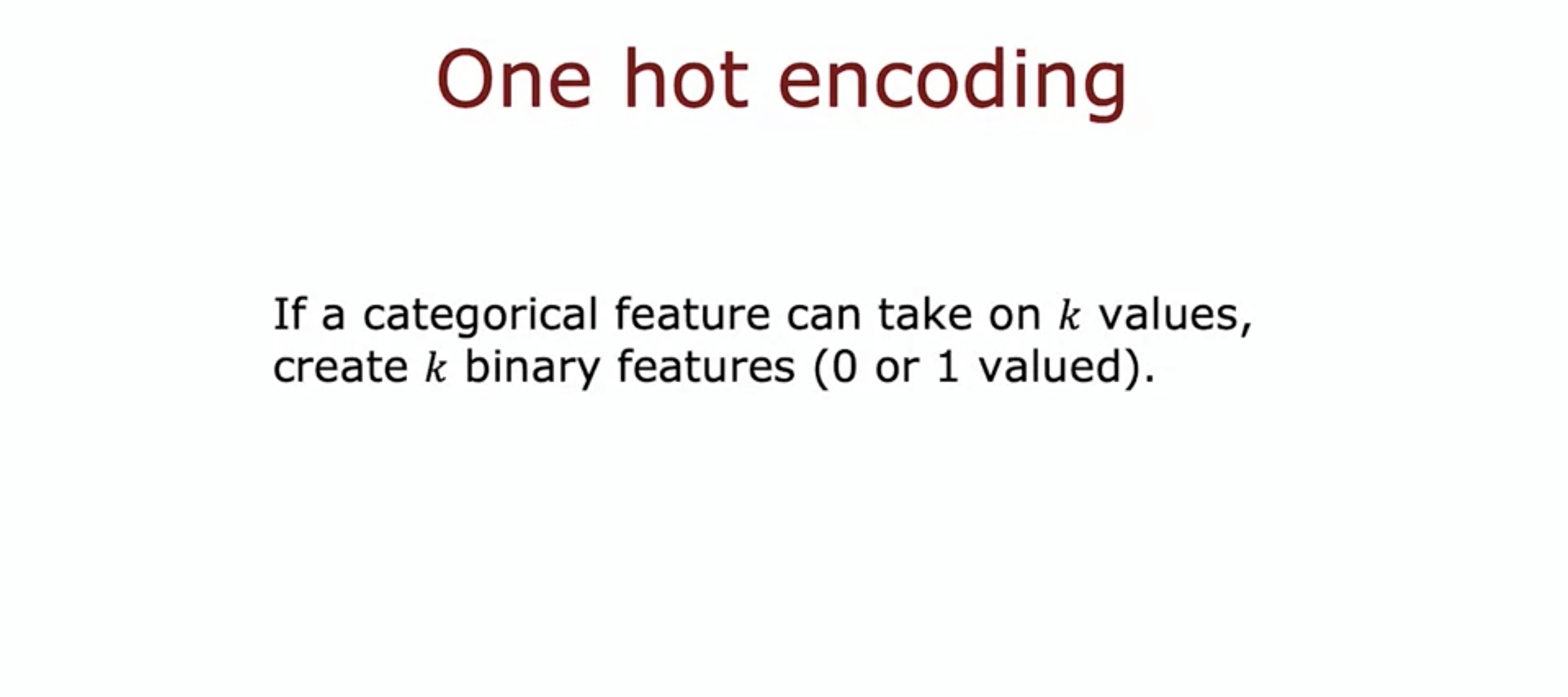
• If a categoricla feature can take on k values (3 ear shapes), then we replace it by creating k binary features (3 features - pointy ears, floppy, oval)

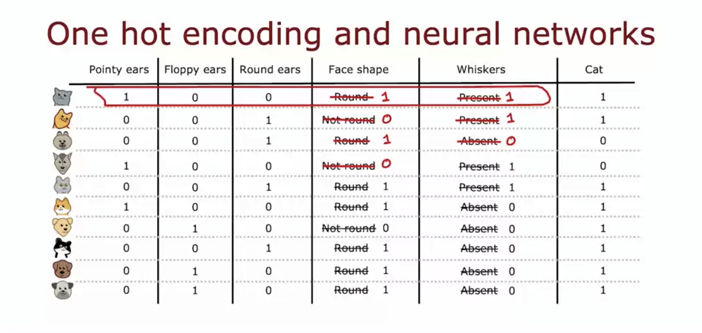
• The face shape and whiskers categorical values are replaced with binary numbers.
• The binary number can then be fed to neural networks as well, not just decision tree.
• These are all discrete values, so binary numbers work.
  • How about for continuous values?

5. Continuous valued features

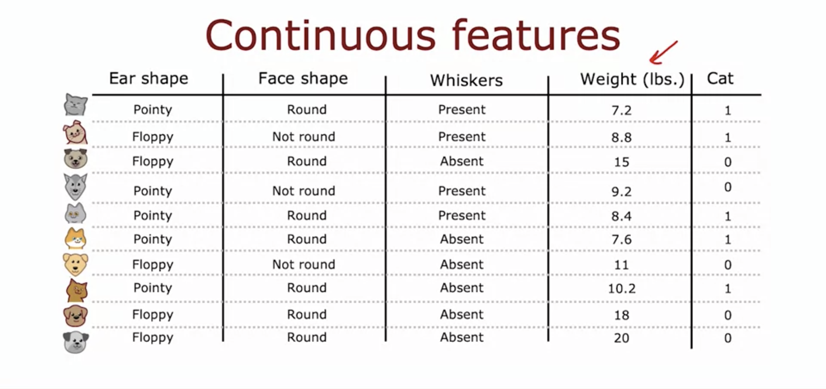
• Now we have a continuous feature, a feature with continuous values - in this case it is the weight of the cat / dog.

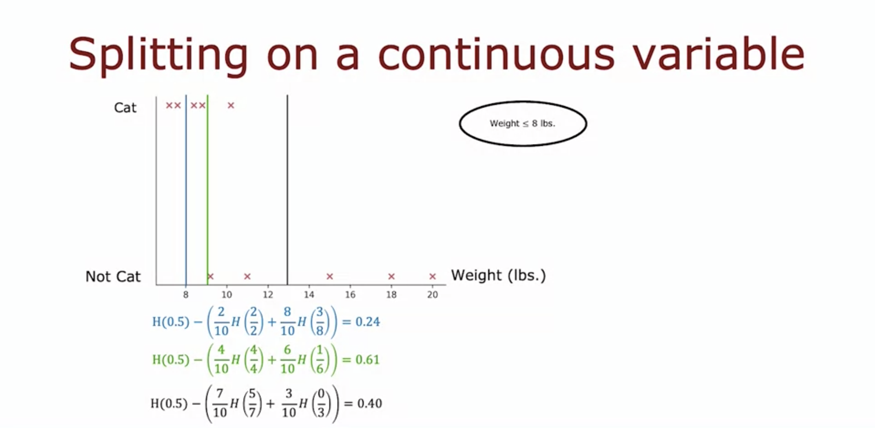
• We can try several threshold values and choose the one that gives the highest information gain.
  • In this case, there are 10 data, so we can try 9 threshold values (because n - 1.)
• Turns out weight that equals to 9 or less is the best threshold value, because it outputs the highest information gain value.