Linear Regression Model

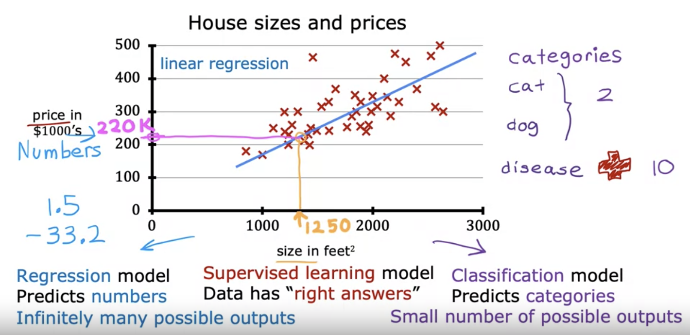
• Linear Regression model: drawing a fitting linear line.

Terminology

• Training set: Data used to train the model.
  • ex: Table of house sizes in feet^2 and prices.
• x = "input" variable feature
• y = "output" / "target" variable
• m = number of training examples
• (x, y) = single training example.
• (x^(i), y^(i)) = ith training example.

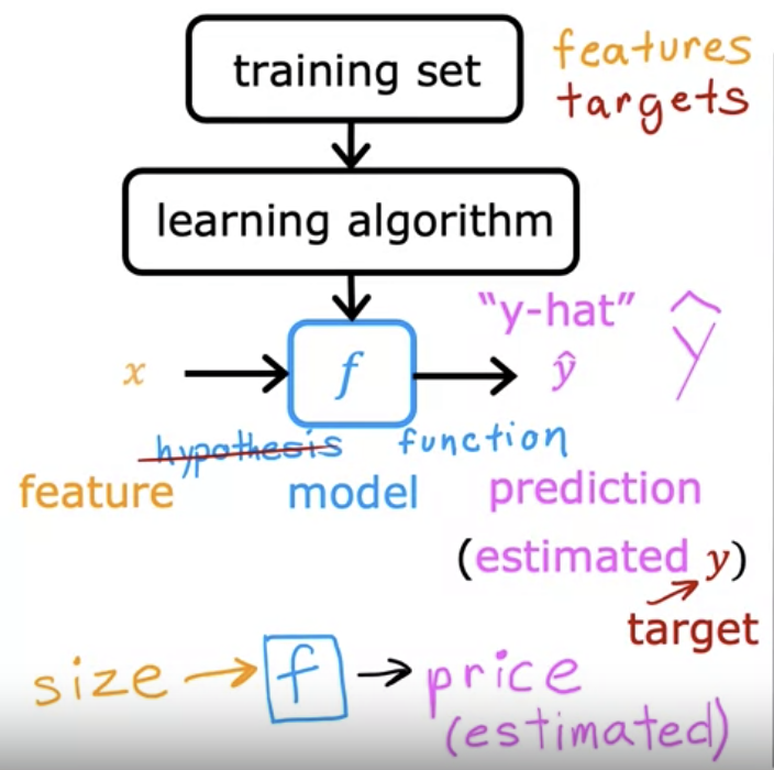
• y-hat refers to the estimated target value.
• y is the "target" value
  
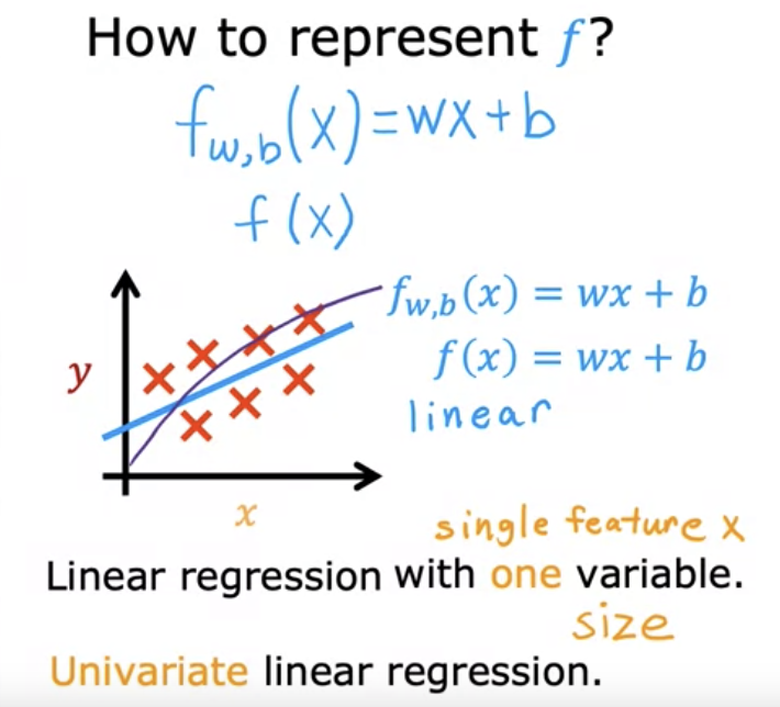
• Linear regression with one variable (x, feature) is called "Univariate linear regression".
• formula: f_w,b(x) = wx + b
  • w and b are called parameters, coefficients, or weights.

Optional Lab: Model Representation

• NumPy - a popular library for scientific computing
• Matplotlib - for plotting data.

import numpy as np
import matplotlib.pyplot as plt
plt.style.use('./deeplearning.mplstyle')

# x_train is the input variable (size in 1000 square feet)
# y_train is the target (price in 1000s of dollars)
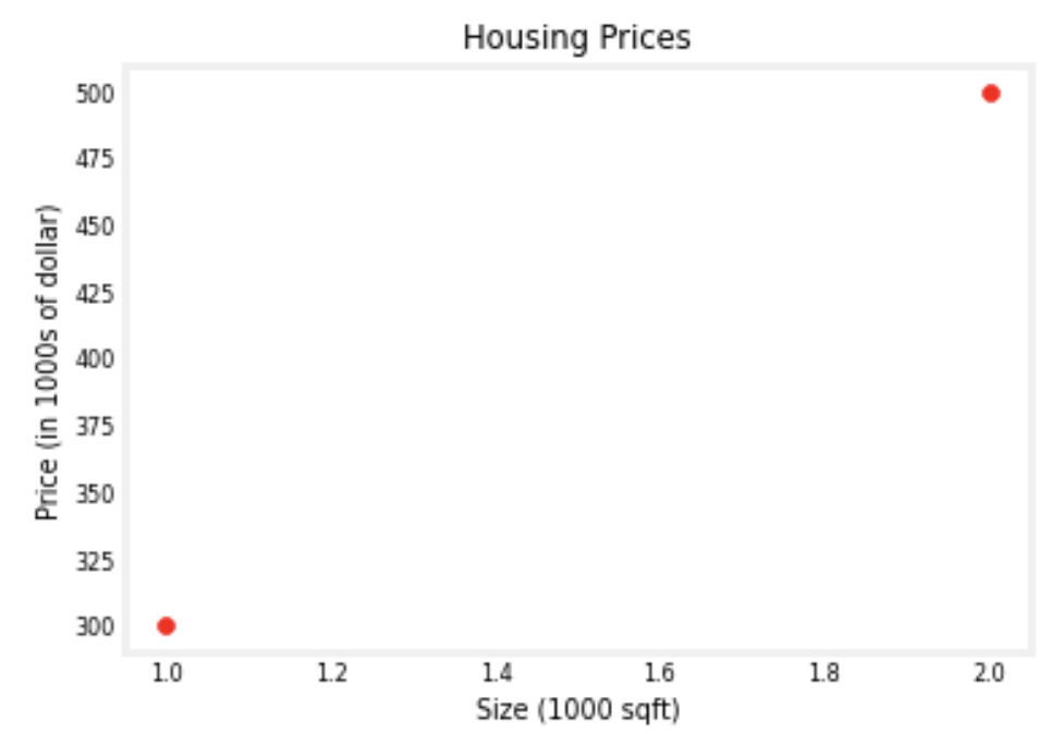
x_train = np.array([1.0, 2.0])
y_train = np.array([300.0, 500.0])
print(f"x_train = {x_train}")
print(f"y_train = {y_train}")

output: x_train = [1. 2.]
y_train = [300. 500.]

• np.array() for storing data set.

# m is the number of training examples
print(f"x_train.shape: {x_train.shape}")
m = x_train.shape[0]
print(f"Number of training examples is: {m}")

output: x_train.shape: (2,)
Number of training examples is: 2

• x_train.shape returns a python tuple with an entry for each dimension.
• x_train.shape[0] is the length of the array.

# m is the number of training examples
m = len(x_train)
print(f"Number of training examples is: {m}")

output: Number of training examples is: 2

i = 0 # Change this to 1 to see (x^1, y^1)

x_i = x_train[i]
y_i = y_train[i]
print(f"(x^({i}), y^({i})) = ({x_i}, {y_i})")

output: (x^(0), y^(0)) = (1.0, 300.0)

# Plot the data points
plt.scatter(x_train, y_train, marker='o', c='r')
# Set the title
plt.title("Housing Prices")
# Set the y-axis label
plt.ylabel('Price (in 1000s of dollar)')
# Set the x-axis label
plt.xlabel('Size (1000 sqft)')
plt.show()

output:

• plt.scatter() to draw scatter plot.
• (self-evident) plt
  • .title()
  • .ylabel()
  • .xlabel()
  • .show()

Model Function:

def compute_model_output(x, w, b):
    """
    Computes the prediction of a linear model
    Args:
      x (ndarray (m,)): Data, m examples 
      w,b (scalar)    : model parameters  
    Returns
      y (ndarray (m,)): target values
    """
    m = x.shape[0]
    f_wb = np.zeros(m)
    for i in range(m):
        f_wb[i] = w * x[i] + b
        
    return f_wb

• np.zeros(m) to fill an array with m number of 0.

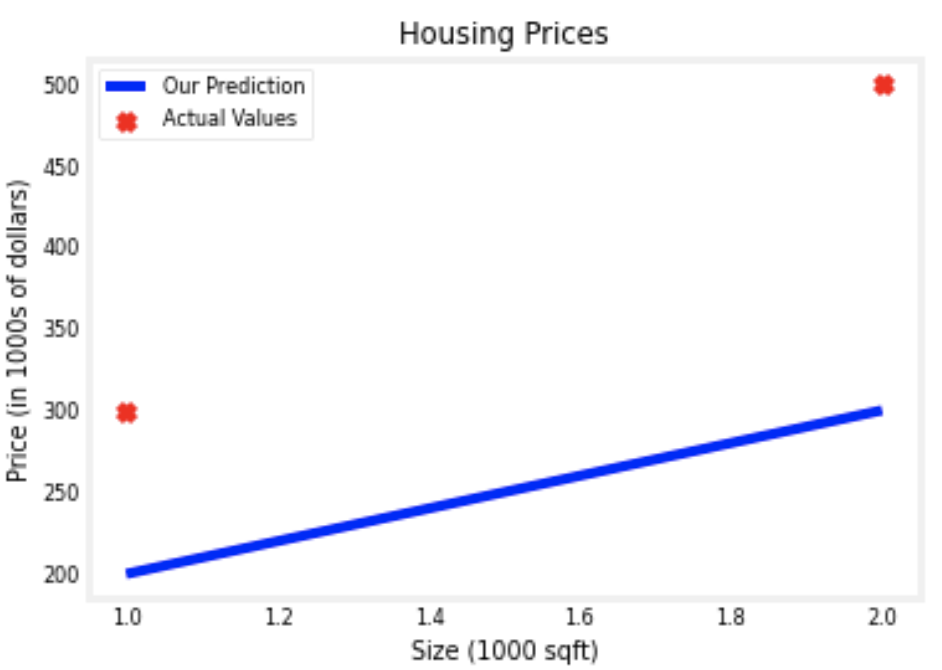
tmp_f_wb = compute_model_output(x_train, w, b,)

# Plot our model prediction
plt.plot(x_train, tmp_f_wb, c='b',label='Our Prediction')

# Plot the data points
plt.scatter(x_train, y_train, marker='x', c='r',label='Actual Values')

# Set the title
plt.title("Housing Prices")
# Set the y-axis label
plt.ylabel('Price (in 1000s of dollars)')
# Set the x-axis label
plt.xlabel('Size (1000 sqft)')
plt.legend()
plt.show()

Output:

• plt.plot(x, y, c="_color", label="_label"): plots the graph.

To make our prediction overlap the data set, w = 200 and b = 100.

w = 200                         
b = 100    
x_i = 1.2
cost_1200sqft = w * x_i + b    

print(f"${cost_1200sqft:.0f} thousand dollars")

Output: $340 thousand dollars

• :.0f - Format float with no decimal places

pi = 3.14159
print(f" pi = {pi:.2f}")

Cost Function

• How far off the prediction is from real value?
• sum of error squared.

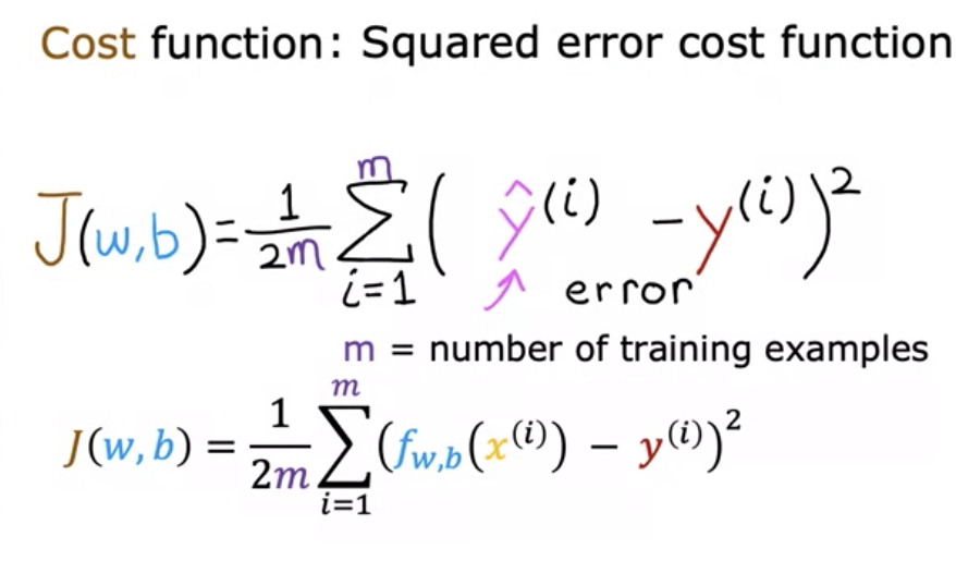
• taking the average of sum of error squared to compute how far off the prediction is.
• J stands for the cost function.

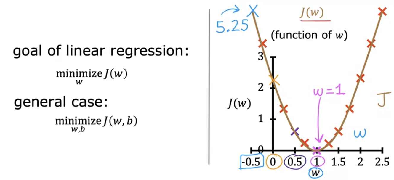
Cost function intuition

• Goal is to minimize J(w, b).

• 3D contour plot
  
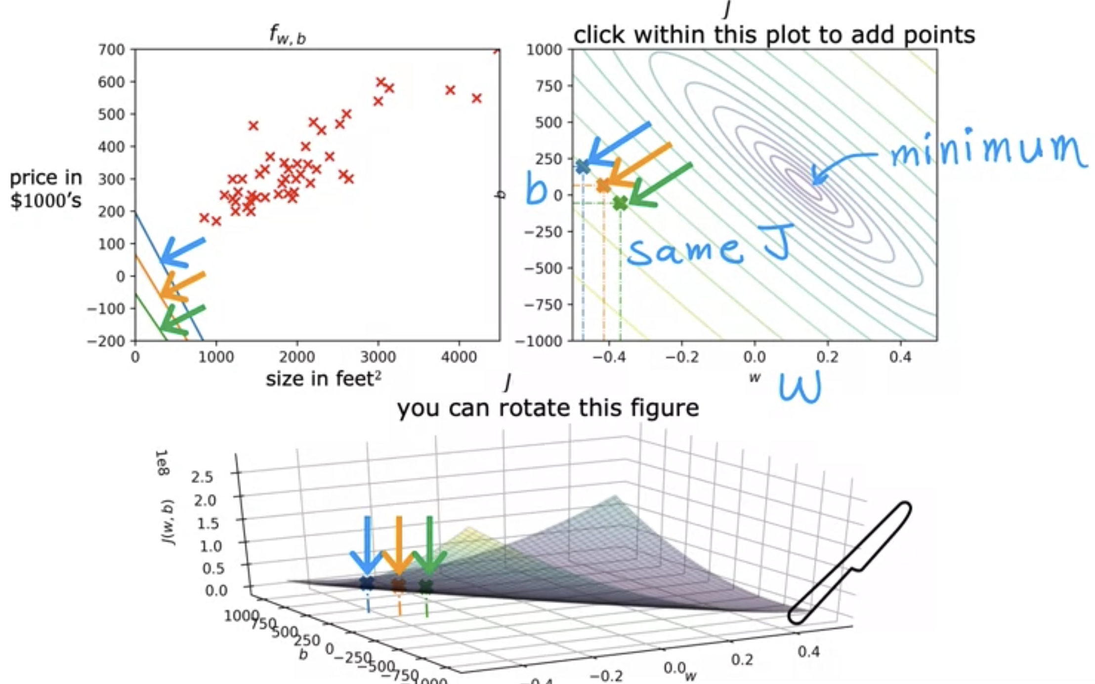
• different colors of rings in a contour plot represent the J values: if the colors are the same, the J values are the same.

Gradient Descent