📖 03장. 케라스와 텐서플로 소개
🗝️ 핵심내용
- 텐서플로, 케라스 그리고 둘 간의 관계 자세히 알아보기
- 딥러닝 작업 환경 설정하기
- 딥러닝의 핵심 개념이 케라스와 텐서플로에 적용되는 방식 소개하기
📑 텐서플로란?
텐서플로(TensorFlow) : 구글에서 만든 파이썬 기반의 무료 오픈 소스 머신 러닝 플랫폼.
텐서플로는 넘파이(NumPy)와 비슷하게 핵심 목적은 수치 텐서에 대한 수학적 표현을 할 수 있는 것.
넘파이와의 차별점
1. 미분 가능한 어떤 표현식에서도 그레이디언트 계산이 가능하므로 머신 러닝에 매우 적합.
2. GPU와 TPU에서도 실행가능.
3. 텐서플로에서 정의한 계산은 여러 머신에 쉽게 분산 가능.
4. 텐서플로 애플리케이션을 실전 환경에 쉽게 배포 가능.
📑 케라스란?
케라스(Keras) : 텐서플로 위에 구축된 파이썬용 딥러닝 API로, 어떤 종류의 딥러닝 모델도 쉽게 만들고 훈련할 수 있는 방법을 제공한다.
케라스는 일관되고 간단한 워크플로를 제공하며, 일반적인 사용에 필요한 작업의 횟수를 최소화하고, 사용자 에러에 대해 명확하고 실행가능한 피드백을 제공한다.
이러한 특징때문에, 입문자부터 전문가까지 비슷한 워크플로를 사용한다.
📑 텐서플로 시작하기
신경망 훈련은 다음과 같은 개념을 중심으로 진행된다.
- 모든 현대적인 머신 러닝의 기초 인프라가 되는 저수준 텐서 연산.
텐서,텐서연산,역전파
- 고수준 딥러닝 개념 (케라스 API)
층,손실 함수,옵티마이저,측정 지표,훈련 루프
상수 텐서와 변수
 # 모두 1 또는 0인 텐서
import tensorflow as tf
x = tf.ones(shape=(2,1))
print(x)
# tf.Tensor(
# [[1.]
#  [1.]], shape=(2, 1), dtype=float32)

x = tf.zeros(shape=(2,1))
print(x)
# tf.Tensor(
# [[0.]
#  [0.]], shape=(2, 1), dtype=float32)

# 랜덤 텐서
x = tf.random.normal(shape=(3,1), mean=0, stddev=1)
print(x)
# tf.Tensor(
# [[ 2.1160586 ]
#  [-0.71148944]
#  [ 1.6094608 ]], shape=(3, 1), dtype=float32)

x = tf.random.uniform(shape=(3,1), minval=0, maxval=1)
print(x)
# tf.Tensor(
# [[0.3348348 ]
#  [0.22721732]
#  [0.54403186]], shape=(3, 1), dtype=float32)
텐서를 만들려면 초깃값이 필요한데, 예를 들어, 모두 1이거나 0인 텐서를 만들거나, 랜텀한 분포에서 뽑은 값으로 텐서를 만들 수 있다.
 # 넘파이 배열에 값 할당하기
import numpy as np
x = np.ones(shape=(2,2))
x[0,0] = 0
print(x)
# [[0. 1.]
#  [1. 1.]]

# 텐서플로 텐서에 값을 할당하지 못함
x = tf.ones(shape=(2,2))
x[0,0] = 0
TypeError: 'tensorflow.python.framework.ops.EagerTensor' object does not support item assignment
넘파이 배열과 텐서플로 텐서의 가장 큰 차이점은 텐서에는 값을 할당할 수 없다는 점이다. 넘파이 배열의 경우 값을 할당할 수 있지만 텐서의 경우 같은 작업을 하면 에러가 발생한다. 이때 tf.Variable을 사용하여 텐서플로 변수를 통해 이러한 작업을 할 수 있다.
# 텐서플로 변수 만들기
v = tf.Variable(initial_value=tf.random.normal(shape=(3,1)))
print(v)
# <tf.Variable 'Variable:0' shape=(3, 1) dtype=float32, numpy=
# array([[-1.0505052],
#        [-0.6222224],
#        [ 1.4685833]], dtype=float32)>

# 텐서플로 변수에 값 할당하기
v.assign(tf.ones((3,1)))
# <tf.Variable 'UnreadVariable' shape=(3, 1) dtype=float32, numpy=
# array([[1.],
#        [1.],
#        [1.]], dtype=float32)>

# 변수 일부에 값 할당하기
v[0,0].assign(3)
# <tf.Variable 'UnreadVariable' shape=(3, 1) dtype=float32, numpy=
# array([[3.],
#        [1.],
#        [1.]], dtype=float32)>

# assign_add() 사용하기
v.assign_add(tf.ones((3,1)))
# <tf.Variable 'UnreadVariable' shape=(3, 1) dtype=float32, numpy=
# array([[4.],
#        [2.],
#        [2.]], dtype=float32)>
다음과 같이 tf.Variable과 assign 메서드를 사용하여 텐서플로 변수의 값을 조작할 수 있다.
GradientTape API 다시 살펴보기
# GradientTape 사용하기
input_var = tf.Variable(initial_value=3.)
with tf.GradientTape() as tape:
    result = tf.square(input_var)
gradient = tape.gradient(result, input_var)
print(gradient)
# tf.Tensor(6.0, shape=(), dtype=float32)

# 상수 텐서 입력과 함께 GradientTape 사용하기
input_const = tf.constant(3.)
with tf.GradientTape() as tape:
	# 상수 텐서의 경우 tape.watch()를 호출하여 추적한다는 것을 수동으로 알려주어야 함.
    tape.watch(input_const)
    result = tf.square(input_const)
gradient = tape.gradient(result, input_const)
print(gradient)
# tf.Tensor(6.0, shape=(), dtype=float32)
텐서플로와 넘파이가 비슷해 보이지만, 텐서플로는 미분 가능한 표현이라면 어떤 입력이라도 그레이디언트를 계산할 수 있다는 기능이 있다. GradientTape 블록을 시작하고 입력 텐서에 대해 결과의 그레이디언트를 구하면 된다.
# 그레이디언트 테이프를 중첩하여 이계도 그레이디언트 계산하기
time = tf.Variable(2.)
with tf.GradientTape() as outer_tape:
    with tf.GradientTape() as inner_tape:
        position = 4.9 * time ** 2
    speed = inner_tape.gradient(position, time)
acceleration = outer_tape.gradient(speed, time)
print(speed, acceleration)
# tf.Tensor(19.6, shape=(), dtype=float32) tf.Tensor(9.8, shape=(), dtype=float32)
위의 예제 코드처럼 이계도, 즉, 그레이디언트의 그레이디언트도 계산할 수 있다.
엔드-투-엔드 예제: 텐서플로 선형 분류기
먼저, 선형적으로 잘 구분되는 합성 데이터를 만들기 위해 특정한 평균과 공분산 행렬을 가진 랜덤한 분포에서 좌표값을 뽑을 것이다. 이러한 작업을 통해 같은 모양을 띄지만 위치만 다른 데이터를 생성할 것이다.
# 2D 평면에 두 클래스의 랜덤한 포인트 생성하기
num_samples_per_class = 1000
negative_samples = np.random.multivariate_normal(
    mean=[0, 3],
    cov=[[1, 0.5],[0.5, 1]],
    size=num_samples_per_class)
positive_samples = np.random.multivariate_normal(
    mean=[3, 0],
    cov=[[1, 0.5], [0.5, 1]],
    size=num_samples_per_class)
먼저, 평균(중심)이 (0,3), (3,0)이고 같은 분산을 가진 데이터를 1000개씩 생성하였다.
# 두 클래스를 (2000, 2) 크기의 한 배열로 쌓기
inputs = np.vstack((negative_samples, positive_samples)).astype(np.float32)
이후, 각 1000개의 데이터를 총 2000개인 한개의 데이터 배열로 쌓는 작업을 하였다.
# (0과 1로 구성된) 타깃 생성하기
targets = np.vstack((np.zeros((num_samples_per_class, 1), dtype="float32"),
                     np.ones((num_samples_per_class, 1), dtype="float32")))
print(targets)
입력 데이터를 생성한 후, 이들을 분류하기 위해 0과 1로 이루어진 label을 생성하였다.
import matplotlib.pyplot as plt

plt.scatter(inputs[:, 0], inputs[:, 1], c=targets[:, 0])
plt.show()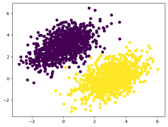
생성한 입력 데이터를 그래프로 나타낸 결과, 의도한 대로 위치만 다르고 모양은 같은 데이터가 잘 생성된 것을 확인 할 수 있다.
이제 두 포인트 클라우드를 구분할 수 있는 선형 분류기를 구현할 것이다. 이 선형 분류기는 하나의 아핀 변환(prediction = W * input + b)이며, 예측과 타깃의 차이를 제곱한 값을 최소화 하도록 훈련될 것이다.
# 선형 분류기의 변수 만들기
input_dim = 2
output_dim = 1
W = tf.Variable(initial_value=tf.random.uniform(shape=(input_dim, output_dim)))
b = tf.Variable(initial_value=tf.zeros(shape=(output_dim,)))
우선, 텐서를 사용하기 위해 초깃값을 설정해 주었다.
# 정방향 패스 함수
def model(inputs):
    return tf.matmul(inputs, W) + b

# 평균 제곱 오차 손실 함수
def square_loss(targets, predictions):
    per_sample_losses = tf.square(targets - predictions)
    return tf.reduce_mean(per_sample_losses)
이후 모델이 주어진 가중치로 예측하고, 이 예측값과 실제값의 차이의 오차값을 구하기 위한 함수를 구현하였다.
# 훈련 스텝 함수
learning_rate = 0.1

def training_step(inputs, targets):
    with tf.GradientTape() as tape:
        predictions = model(inputs)
        loss = square_loss(targets, predictions)
    grad_loss_wrt_W, grad_loss_wrt_b = tape.gradient(loss, [W, b])
    W.assign_sub(grad_loss_wrt_W * learning_rate)
    b.assign_sub(grad_loss_wrt_b * learning_rate)
    return loss
이후, 계산한 손실값을 최소화하기 위하여 손실 함수의 그레이디언트를 계산하고 가중치를 업데이트하기 위해 tf.GradientTape를 사용하여 각 훈련 스텝에서 수행할 함수를 구현하였다.
# 배치 훈련 루프
for step in range(40):
    loss = training_step(inputs, targets)
    print(f'{step}번째 스텝의 손실: {loss:.4f}')
# 0번째 스텝의 손실: 7.2605
# 1번째 스텝의 손실: 1.0902
# ...
# 38번째 스텝의 손실: 0.0313
# 39번째 스텝의 손실: 0.0308
40번의 에포크 후 손실 값이 점차 줄어들어 0.03에서 안정화되는 것을 확인할 수 있었다.
# 훈련 입력에 대한 모델의 예측
predictions = model(inputs)
plt.scatter(inputs[:, 0], inputs[:, 1], c=predictions[:, 0] > 0.5)
plt.show()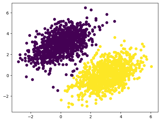
학습된 모델이 훈련데이터에 대해 어떻게 예측하는지 그래프로 나타내었다.
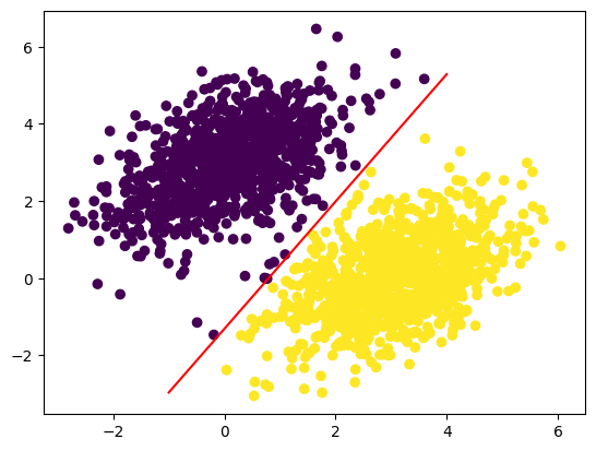
# 직선으로 나타낸 선형 모델
x = np.linspace(-1, 4, 100)
y = -W[0] / W[1] * x + (0.5 - b) / W[1]
plt.plot(x, y, "-r")
plt.scatter(inputs[:, 0], inputs[:, 1], c=predictions[:, 0] > 0.5)
plt.show()
이때, 포인트 [x, y]에 대한 값은
prediction == [[w1], [w2]] dot [x, y] + b == w1 * x + w2 * y + b 인데,
클래스 0은 w1 * x + w2 * y + b < 0.5 이고
클래스 1은 w1 * x + w2 * y + b > 0.5 로 정의할 수 있다.
이때 실제로 찾고자 하는 것은 평면 위의 직선의 방정식
w1 * x + w2 * y + b = 0.5 가 되고, 이 직선보다 위에 있으면 클래스 1, 아래에 있으면 클래스 0이다.
위의 방정식을 정리하면
y = -w1 / w2 * x + (0.5 - b) / w2 가 되고, 이를 평면에 아래와 같이 그릴 수 있다.
📑 신경망의 구조: 핵심 Keras API 이해하기
이제 딥러닝 모델을 구축하는 데 더 생산적이고 강력한 방법인 케라스 API를 배워보자.
층: 딥러닝의 구성 요소
층(layer) : 신경망의 기본 데이터 구조로, 하나 이상의 텐서를 입력으로 받고 하나 이상의 텐서를 출력하는 데이터 처리 모듈이다.
층은 대부분의 경우 가중치(weight)라는 층의 상태를 가지는데, 가중치는 확률적 경사 하강법으로 학습되는 하나 이상의 텐서이며 여기에 신경망이 학습한 지식이 담겨있다.
# Layer의 서브 클래스(subclass)로 구현한 Dense 층
import tensorflow as tf
from tensorflow import keras

class SimpleDense(keras.layers.Layer):
    def __init__(self, units, activation=None):
        super().__init__() # 부모의 속성을 모두 물려받음
        self.units = units
        self.activation = activation

    def build(self, input_shape):
    	# 입력의 크기에 맞춰 동적으로 shape 생성
        input_dim = input_shape[-1]
        self.W = self.add_weight(shape=(input_dim, self.units),
                                 initializer="random_normal")
        self.b = self.add_weight(shape=(self.units,),
                                 initializer='zeros')

    def call(self, inputs):
        y = tf.matmul(inputs, self.W) + self.b
        if self.activation is not None:
            y = self.activation(y)
        return y

# 클래스 인스턴스 생성
my_dense = SimpleDense(units=32, activation=tf.nn.relu)
input_tensor = tf.ones(shape=(2, 784))
output_tensor = my_dense(input_tensor)
print(output_tensor.shape) # (2, 32)
이때 층을 호출하기 위해 __call__() 메서드를 이용하여 호출하였는데 클래스 내부에 call() 과 build() 메서드는 왜 구현했을까?
이는 때에 맞추어 가중치를 생성해야하기 때문이다. 또한 케라스의 기본 Layer 클래스의 속성을 그대로 물려받기 때문에 생성 시 기본 Layer 클래스의 __call__() 메서드를 통해 호출된다.
# SimpleDense 클래스에서 __call()__ 메서드가 아닌 call() 사용한 이유
# 기본 Layer 클래스의 속성을 모두 물려받았기 때문이다.
# 기본 Layer 클래스가 호출되면 내부적으로 build()와 call() 호출!
def __call__(self, inputs):
    if not self.built:
        self.build(inputs.shape) # 자동 크기 추론 작업
        self.built = True
    return self.call(inputs)
이처럼 기본 Layer 클래스의 __call__() 메서드가 자동으로 입력의 크기를 추론하는 작업을 해준다.
'컴파일' 단계: 학습 과정 설정
위에서 다룬 층을 쌓아 모델 구조를 정의한 뒤, 다음 세가지를 더 선택해야한다.
손실 함수(loss function) : 훈련 과정에서 최소화할 값.
옵티마이저(optimizer) : 손실 함수를 기반으로 네트워크가 어떻게 업데이트될지 결정.
측정 지표(metric) : 훈련과 검증 과정에서 모니터링할 성공의 척도.
위 세가지를 선택했다면 모델에 내장된 compile()과 fit() 메서드를 사용하여 모델 훈련을 시작할 수 있다.
fit() 메서드 이해하기
compile() 다음에는 fit() 메서드를 호출하여 훈련 루프를 구현한다. 다음은 fit() 메서드의 주요 매개변수로는 훈련할 데이터(입력과 타깃)와 훈련할 에포크(epoch) 횟수, 각 에포크에서 사용할 배치 크기가 있다.
model = keras.Sequential([keras.layers.Dense(1)])
model.compile(optimizer=keras.optimizers.RMSprop(learning_rate=0.1),
              loss=keras.losses.MeanSquaredError(),
              metrics=[keras.metrics.BinaryAccuracy()])

# 검증데이터에 한 클래스의 샘플만 포함되는 것을 막기위해 입력과 타깃을 섞는다.
indices_permutation = np.random.permutation(len(inputs))
shuffled_inputs = inputs[indices_permutation]
shuffled_targets = targets[indices_permutation]

# 훈련 입력과 타깃의 30%를 검증용으로 떼어놓는다.
num_validation_samples = int(0.3 * len(inputs))
val_inputs = shuffled_inputs[:num_validation_samples]
val_targets = shuffled_targets[:num_validation_samples]
training_inputs = shuffled_inputs[num_validation_samples:]
training_targets = shuffled_targets[num_validation_samples:]

model.fit(
    training_inputs,
    training_targets,
    epochs=5,
    batch_size=128,
    validation_data=(val_inputs, val_targets)
)
fit() 메서드를 호출하기 전에 훈련데이터의 일부를 검증데이터로 분리하여 훈련과정에서 검증 손실 값을 계산하는데 사용할 수 있다. 머신 러닝의 목표는 훈련 데이터에서 잘 작동하는 모델을 만드는 것이 아닌, 범용적으로 잘 동작하는 모델을 얻는 것이기 때문에 훈련 과정에서 사용하지 않은 데이터를 잘 예측하는 것이 중요하다. 따라서 검증데이터를 사용하여 훈련데이터가 아닌 새로운 데이터에서의 예측에 대한 손실 값을 사용하여 모델을 검증할 수 있다.
loss_and_metrics = model.evaluate(val_inputs, val_targets, batch_size=128)
print(loss_and_metrics)
# [0.11686566472053528, 0.8983333110809326]
또한, evaluate() 메서드를 사용하여 훈련이 끝난 후 검증 손실과 측정 지표를 계산할 수도 있다.
추론: 훈련한 모델 사용하기
predictions = model.predict(new_inputs, batch_size=128)마지막으로, predict() 메서드를 호출하여 실제 예측하고자 하는 값에 대한 모델의 예측값을 계산할 수 있다.
🔗 출처
https://www.gilbut.co.kr/book/view?bookcode=BN003496