📦 Lab: CNN on CIFAR 100 data

# Read the CIFAR100 data, which is available in the torchvision package
(cifar_train, cifar_test) = [
    CIFAR100(root="data", train=train, download=True)
    for train in [True, False]
]

transform = ToTensor()

cifar_train_X = torch.stack([transform(x) for x in cifar_train.data])
cifar_test_X  = torch.stack([transform(x) for x in cifar_test.data])

cifar_train = TensorDataset(cifar_train_X, torch.tensor(cifar_train.targets))
cifar_test  = TensorDataset(cifar_test_X, torch.tensor(cifar_test.targets))

print(cifar_train_X.shape)  # torch.Size([50000, 3, 32, 32])

The CIFAR100 dataset consists of:

• 50,000 training images and 10,000 test images
• Each image is represented as a 3D tensor of shape (3, 32, 32), where:
  • 3 is the number of color channels (RGB)
  • 32 x 32 is the height and width in pixels

즉, 각 이미지는 RGB 컬러 이미지이며, 총 100개 클래스로 분류되는 구조입니다.

# Create the data module
max_num_workers = rec_num_workers()
print(max_num_workers)  # 2

cifar_dm = SimpleDataModule(
    cifar_train,
    cifar_test,
    validation=0.2,
    num_workers=max_num_workers,
    batch_size=128
)

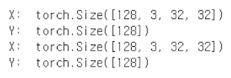
for idx, (X_, Y_) in enumerate(cifar_dm.train_dataloader()):
    print('X: ', X_.shape)
    print('Y: ', Y_.shape)
    if idx >= 1:
        break

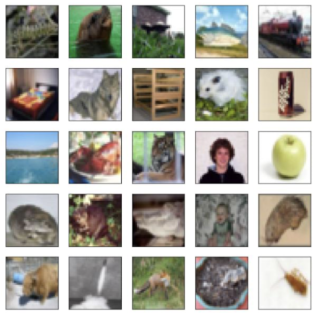
# Choose random images from the training data
fig, axes = subplots(5, 5, figsize=(10, 10))
rng = np.random.default_rng(4)
indices = rng.choice(np.arange(len(cifar_train)), 25, replace=False).reshape((5, 5))

for i in range(5):
    for j in range(5):
        idx = indices[i, j]
        axes[i, j].imshow(
            np.transpose(cifar_train[idx][0], [1, 2, 0]),
            interpolation=None
        )
        axes[i, j].set_xticks([])
        axes[i, j].set_yticks([])

# Specify a moderately-sized CNN
class BuildingBlock(nn.Module):
    def __init__(self, in_channels, out_channels):
        super(BuildingBlock, self).__init__()
        self.conv = nn.Conv2d(
            in_channels=in_channels,
            out_channels=out_channels,
            kernel_size=(3, 3),
            padding='same'
        )
        self.activation = nn.ReLU()
        self.pool = nn.MaxPool2d(kernel_size=(2, 2))

    def forward(self, x):
        return self.pool(self.activation(self.conv(x)))

padding='same' 인자는 nn.Conv2d() 에서 입력과 출력의 공간 차원(Height, Width)을 동일하게 유지해 주는 역할을 합니다.
즉, 커널이 이미지의 가장자리를 벗어나지 않도록 필요한 만큼의 제로 패딩(zero-padding) 을 자동으로 적용합니다.

✅ 이렇게 하면 convolution 연산 후에도 feature map의 크기가 줄어들지 않아, 네트워크 설계가 단순해지고 feature dimension 추적이 쉬워집니다.

# Form the deep learning model for CIFAR100 data
# We use several BuildingBlock() modules sequentially

class CIFARModel(nn.Module):
    def __init__(self):
        super(CIFARModel, self).__init__()
        sizes = [(3, 32), (32, 64), (64, 128), (128, 256)]
        
        self.conv = nn.Sequential(
            *[BuildingBlock(in_, out_) for in_, out_ in sizes]
        )
        
        self.output = nn.Sequential(
            nn.Dropout(0.5),
            nn.Linear(2 * 2 * 256, 512),
            nn.ReLU(),
            nn.Linear(512, 100)
        )

    def forward(self, x):
        val = self.conv(x)
        val = torch.flatten(val, start_dim=1)
        return self.output(val)

# Build the model and look at the summary
cifar_model = CIFARModel()

summary(
    cifar_model,
    input_data=X_,
    col_names=['input_size', 'output_size', 'num_params']
)

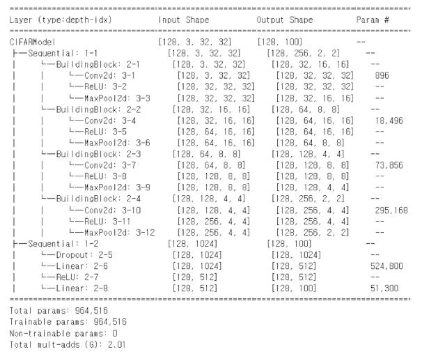해당 모델에서 학습 가능한 파라미터 수는 총 964,516개

# Create the data module
cifar_optimizer = RMSprop(cifar_model.parameters(), lr=0.001)

cifar_module = SimpleModule.classification(
    cifar_model,
    num_classes=100,
    optimizer=cifar_optimizer
)

cifar_logger = CSVLogger('logs', name='CIFAR100')

cifar_trainer = Trainer(
    deterministic=True,
    max_epochs=30,
    logger=cifar_logger,
    callbacks=[ErrorTracker()]
)

cifar_trainer.fit(cifar_module, datamodule=cifar_dm)

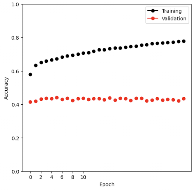
# Check validation and training accuracy
log_path       = cifar_logger.experiment.metrics_file_path
cifar_results  = pd.read_csv(log_path)

fig, ax        = subplots(1, 1, figsize=(6, 6))
summary_plot(cifar_results,
             ax,
             col='accuracy',
             ylabel='Accuracy')

ax.set_xticks(np.linspace(0, 10, 6).astype(int))
ax.set_ylabel('Accuracy')
ax.set_ylim([0, 1])

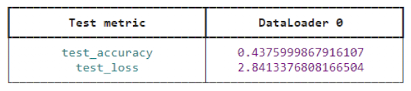
# Evaluate our model on our test data
cifar_trainer.test(cifar_module, datamodule=cifar_dm)

---

📦 Lab: Using Pretrained CNN Models

# Hardware Acceleration
try:
    for name, metric in cifar_module.metrics.items():
        cifar_module.metrics[name] = metric.to('mps')

    cifar_trainer_mps = Trainer(
        accelerator='mps',
        deterministic=True,
        max_epochs=30
    )

    cifar_trainer_mps.fit(cifar_module, datamodule=cifar_dm)
    cifar_trainer_mps.test(cifar_module, datamodule=cifar_dm)

except:
    pass

Trainer 호출 방식과 평가할 metric 설정을 변경함으로써, 학습 속도가 2~3배 빨라지는 효과를 얻을 수 있다.
→ 즉, 에폭당 연산 효율이 크게 향상되며, 동일한 모델이라도 더 빠르게 학습 가능해진다는 뜻이다.

# Use Pretrained CNN Models
from google.colab import drive
drive.mount('/content/drive')

import os
print(os.listdir('/content/drive/MyDrive'))

resize     = Resize((232, 232), antialias=True)
crop       = CenterCrop(224)
normalize  = Normalize([0.485, 0.456, 0.406],
                       [0.229, 0.224, 0.225])

imgfiles = sorted([
    f for f in glob('/content/drive/MyDrive/book_images/*')
])

imgs = torch.stack([
    torch.div(crop(resize(read_image(f))), 255)
    for f in imgfiles
])

imgs = normalize(imgs)
imgs.size()

torch.Size([6, 3, 224, 224])

# Set up the trained network with the weights
resnet_model = resnet50(weights=ResNet50_Weights.DEFAULT)

summary(resnet_model,
        input_data=imgs,
        col_names=['input_size', 'output_size', 'num_params'])

# Set the mode to eval() to ensure that the model is ready to predict on new data.
resnet_model.eval()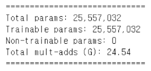

# Feed our six images through the fitted network
img_preds = resnet_model(imgs)
img_probs = np.exp(np.asarray(img_preds.detach()))
img_probs /= img_probs.sum(1)[:, None]

# Download the index file associated with ImageNet
labs = json.load(open('/content/drive/MyDrive/book_images/imagenet_class_index.json'))
class_labels = pd.DataFrame([(int(k), v[1]) for k, v in labs.items()],
                            columns=['idx', 'label'])
class_labels = class_labels.set_index('idx')
class_labels = class_labels.sort_index()

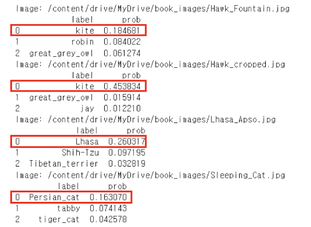
# Construct a data frame for each image file with the
labels with the three highest probabilities as estimated
by the model above.
for i, imgfile in enumerate(imgfiles):
img_df = class_labels.copy()
img_df['prob'] = img_probs[i]
img_df = img_df.sort_values(by='prob',
ascending=False)[:3]
print(f'Image: {imgfile}')
print(img_df.reset_index().drop(columns=['idx']))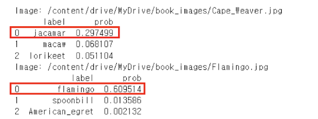