참고
이전 Object Detection에 대해 정리한 포스팅이 있습니다.😃
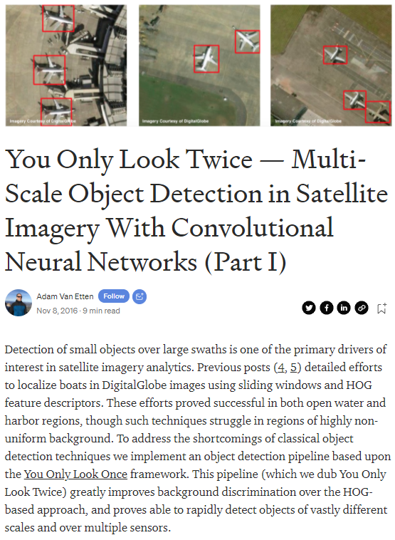
이번에 리뷰할 글은 You Only Look Twice — Multi-Scale Object Detection in Satellite Imagery With Convolutional Neural Networks (Part I)이란 제목의 글입니다.
원래는 You Only Look Once로 줄여서 YOLO라는 모델이었는데 이번엔 You Only Look Twice입니다! YOLT라고 부르는 것 같습니다. 이름 그대로 한 번이 아니라 두 번 봤다는 의미일까요?🙂
❗ YOLO에 대해 정리한 글도 있습니다 - [논문 리뷰] You Only Look Once - YOLO v1 (+ v2, v3)
Conv Neural Networks를 통해 위성 영상에서 여러 개의 object detection을 수행하는 것에 대한 게시글입니다.
넓은 범위에서 작은 객체(small object)를 탐지하는 것은 위성 영상 분석 중 주요 관심사입니다.
이전 게시물 [4], [5]에서는 sliding windows와 HOG feature descriptors를 통해 DigitalGlobe 이미지에서 boat를 localize하려는 노력을 설명했다고 합니다.
Conv Neural Networks(Faster RCNN, YOLO)를 이용한 다수의 파이프라인은 open water와 harbor regions에서의 object detection을 성공적으로 증명하였지만, 이 기술은 큰 이미지에서 small object를 탐지하는데 최적화 되지 않았으며 종종 성능이 좋지 않았습니다. 또한, background가 균일하지 않은 지역에서 어려움을 겪습니다.
이러한 기존 object detection 기술의 단점을 해결하기 위해 You Only Look Once 프레임워크를 기반으로 object detection pipeline을 구현합니다.
이 pipeline은 You Only Look Twice이라고 하고, HOG 기반 접근 방식에 대한 배경 식별을 크게 개선하고, 여러 센서에서 매우 다른 축적의 object를 빠르게 감지할 수 있음을 입증했습니다!
1. Satellite Imagery Object Detection Overview
ImageNet 대회는 CV object detection 분야에서 빠른 발전에 도움이 되었습니다. 그러나 ImageNet의 dataset과 위성 영상 사이에는 몇 가지 차이가 있습니다.
4가지 문제가 어려움을 낳습니다.
- 위성 영상에서 object는 매우 작다(20 pixels 이하)
- 단위 원을 기준으로 회전한다.(rotated)
- Input image는 매우 크다. (주로 hundreds of megapixels)
- training data가 많이 부족하다.
그러나 object의 physical한 scale과 pixel scale을 미리 알고 있으면 관찰하는 각도의 편차가 적습니다. 마지막으로 주목해야 할 문제는 수백 킬로 미터 떨어진 곳에서 관측한 것이 때때로 함정에 빠지게 할 수 있습니다.(잘못 탐지하는 경우!)
실제로 2016년 10월 13일 New York Times의 1면에는 러시아 무기 모형에 대한 기사가 실렸습니다.
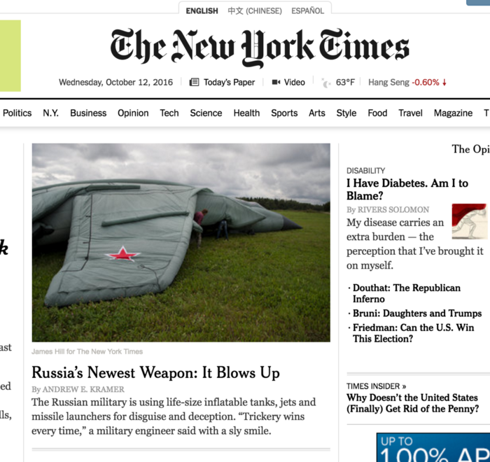
Figure 1. Screenshot of The New York Times on October 13, 2016 showing inflatable Russian weapons mock-ups designed to fool remote sensing apparatus.
2. HOG Boat Detection Challenges
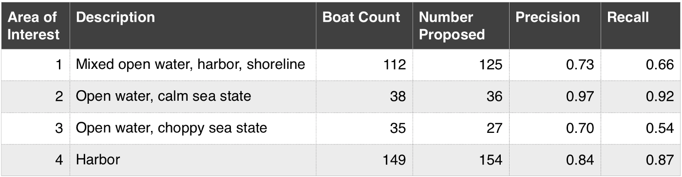
[4] Figure 9. Object detection performance for each of the four areas of interest.
HOG + Sliding Window의 object Detection은 'open water and harbor'에서 좋은 결과를 보여주었습니다. (F1 ~ 0.9)
또한, F1 score는 precision과 recall의 조화 평균이며 0(모든 예측이 잘못됨)에서 1(완벽한 예측)까지 다양합니다.
HOG + Sliding Window의 파이프라인의 한계를 탐색하기 위해 background가 덜 균일하고 다른 센서에서 적용해 봅니다.
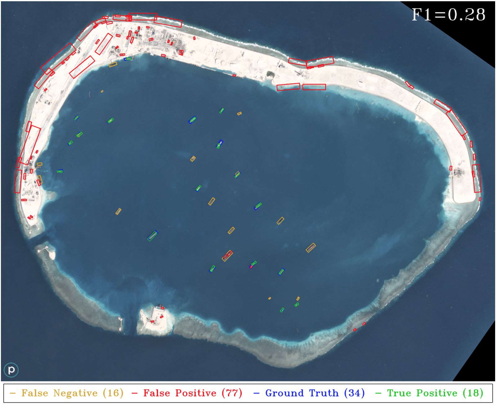
Figure 2. HOG + Sliding Window results applied to a different sensor (Planet) than the training data corpus (DigitalGlobe).
위 test 이미지는 3m GSD의 planet 이미지지만, classifier는 0.5m GSD의 DigitalGlobe data에 대해 훈련되었다고 합니다.
※ 용어 정리
- Spatial resolution(공간 해상도): 영상/이미지를 공간영역상에서 얼마나 자세하게 표현할 수 있는가의 척도
- GSD: Ground Sample Distance이며, 영상에서 한 픽셀에 해당하는 실제 거리를 의미
- GRD: Ground Resolved Distance이며, 두 물체를 구분할 수 있는 최소한의 거리를 의미
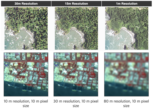
윗줄은 GSD를 각각 30m, 15m, 1m에 해당하며, 한 pixel당 갖는 거리가 작을 수록 더 선명하게 느껴집니다. GRD도 같은 값을 가집니다. 이 경우를 full resolution이라고 합니다.
아랫줄은 GSD가 모두 10m이지만, GRD는 각각 10m, 30m, 80m의 값을 가집니다. GRD 값이 클수록 더 흐리게 보이는 것을 알 수 있습니다. 해상도가 나빠진다는 것을 의미합니다.
pixel 크기 자체는 작지만 각 픽셀이 하나의 물체를 뜻하는 것이 아니고, 물체 간의 거리가 30m, 80m 떨어져 있어야 물체 구분이 가능하다는 의미입니다.
GRD 값은 GSD보다 값이 크거나 같을 수 밖에 없고, 대부분 동일하며 해당 영상 공간 해상도라고 말한다고 합니다!
출처: https://blog.si-analytics.ai/56
3. Object Detection With Deep Learning
여기서는 YOLO(You Only Look Once)의 Framework를 적용하여 위성 영상에서 object detection을 수행합니다. YOLO는 single Convolutional Neural Network를 사용하여 class와 Bbox를 예측합니다.
이 네트워크는 train, test 시간에 이미지 전체를 보고, contextual 정보를 인코딩하므로
background를 식별하는 성능이 크게 향상됩니다. GoogLeNet의 아키텍처를 활용하고 작은 input test image에 대해 real-time 속도로 실행됩니다. background 정보를 캡처하는 기능과 결합된 이 접근 방식의 빠른 속도는 위성 영상과 함께 사용됩니다.
sliding window와 결합된 CNN classifier는 인상적인 결과를 얻을 수 있지만, 빠르게 계산하기 어렵습니다. GoogLeNet 기반 classifier를 평가하는 것은 HOG 기반 classifier보다 hardware에서 50배 느립니다.
sliding window의 cutouts의 또 다른 단점은 이미지의 아주 작은 부분만 보기 때문에 유용한 background의 정보를 버리게 됩니다. YOLO freamwork는 background 식별 문제를 해결하고 CNN + Sliding Window 접근 방식보다 대규모 데이터 세트로 훨씬 더 잘 확장됩니다!
※ Sliding Window의 개념
sliding window의 접근 방식은 원하는 크기의 Bbox가 test image를 가로질러 slide하고 각 위치에서 현재 slide에 이미지 classifier를 적용합니다.
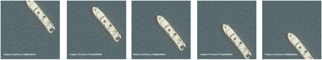
[4] Figure 5. Sliding window shown iterating across an image (left). A liberal image classifier is applied to these cutouts and anything resembling a boat is saved as a positive (right) (Imagery Courtesy of DigitalGlobe).
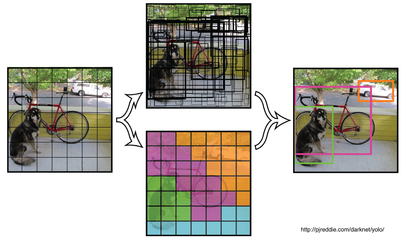
Figure 3. Illustration of the default YOLO framework. The input image is split into a 7x7 grid and the convolutional neural network classifier outputs a matrix of bounding box confidences and class probabilities for each grid square. These outputs are filtered and overlapping detections suppressed to form the final detections on the right.
그러나 이 framework는 몇 가지 제약이 있으며 논문에도 요약되었습니다.
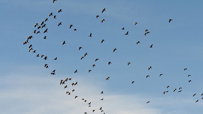
- “Our model struggles with small objects that appear in groups, such as flocks of birds”
- 우리 모델은 새 떼처럼 그룹으로 나타나는 small object로 어려움을 겪습니다.
- “It struggles to generalize objects in new or unusual aspect ratios or configurations”
- 새롭거나 특이한 종횡비 구성은 개체를 일반화(generalize)하는데 어려움을 겪습니다.
- “Our model uses relatively coarse features for predicting bounding boxes since our architecture has multiple downsampling layers from the original image”
- 우리 모델은 원본 이미지에 여러 downsampling layer들이 있기 때문에 Bbox를 예측하기 위해 상대적으로 coarse features를 사용합니다. 실제로 input image를 더 크게 resize하여 input image로 넣어줍니다.
이 문제를 해결하기 나온 것이 YOLOT!!!!!!!!!!!!!!!!! 입니다. You Only Look Twice! 이름의 이유는 나중에 밝힌다고 하네요.

1번의 문제점은 작으면서 모여 있는 새 떼 같은 object를 detection하기에 어려움을 겪는다는 거였습니다.
- 작은 object를 찾기 위해 sliding window를 통해 Upsampling하는 방법
- 여러 scale에서 detector의 ensemble 실행
2번의 문제점은 genearalize 문제였습니다.
- training data를 Augmenatation하는 방법(re-scaling and rotations)
3번의 문제점은 downsampling 문제로 coarse features를 사용하는 문제였습니다.
- 최종 Conv layer가 더 조밀한 grid를 가지도록 새로운 network architecture를 정의합니다.
YOLT framework의 output은 아주 큰 test image에서 다양한 image chip에 대한 결과의 ensemble을 결합하기 위해 후처리 됩니다. 이러한 수정은 44 FPS에서 18 FPS로 줄입니다.
구현해야 하는 매우 조밀한 grid에 대해 많은 parameter는 이 크기보다 더 큰 이미지에 대해 하드웨어 용량을 초과히시킵니다. 최대 이미지 크기가 2-4배로 커질 수 있다는 점을 유의해야 한다고 하네요.
4. YOLT Training Data
train data는 DigitalGlobe and Planet에서 large image의 small chip에서 수집됩니다. Label은 각 object에 대한 Bbox와 category identifier로 구성됩니다.
여기서는 네 가지 category에 집중합니다.
- Boats in open water
- Boats in harbor
- Airplanes
- Airports
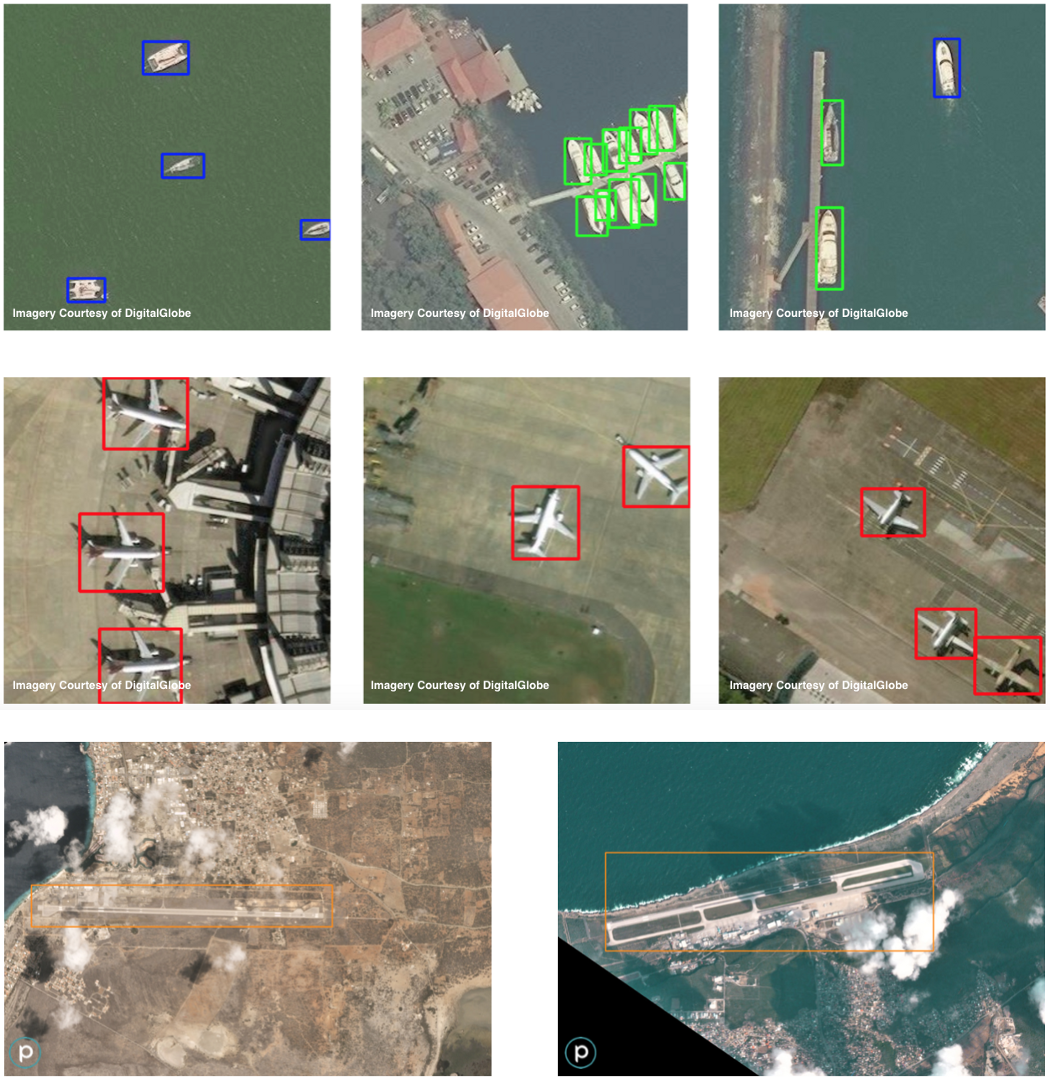
Figure 4. YOLT Training data. The top row displays labels for boats in harbor (green) and open water (blue) for DigitalGlobe data. The middle row shows airplanes (red) in DigitalGlobe data. The bottom row shows airports and airfields (orange) in Planet data.
네 카테고리 이미지에 labeling하고 평균 몇 개의 object를 찾았다는 내용입니다. 마지막 이미지는 공항으로 단 일 Bbox만 존재합니다.
Part 1에서는 boat와 airplane에 대해서만 train하고 part 2에서 airports and airfields를 다룬다고 합니다.
YOLT 구현을 위해 2가지 sclae로 large test image에 sliding window를 실행합니다. 하나는 소형 boat와 airplane을 위한 120m window이고, 하나는 대형 vessel과 airliner를 위한 225m window입니다.
YOLT는 speed보다 accuracy를 maximize하도록 만들어졌습니다. 속도를 높이는 방법으로는 a single sliding window size를 사용하거나 이미지를 downsampling하여 sliding window의 크기를 늘리면 개선됩니다.
그렇지만 우리는 매우 작은 object를 찾고 있기 때문에 관심 있는 object(15m boats)와 background object(15m building)를 식별하는 성능에 부정적인 영향을 미칩니다.
5. YOLT Object Detection Results
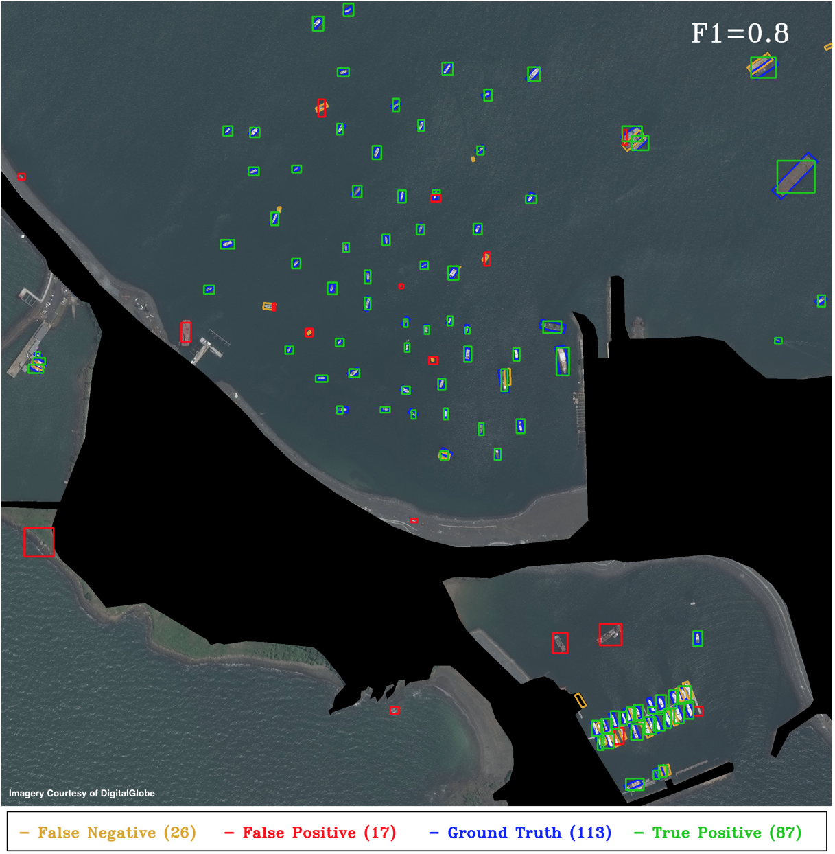
Figure 6. YOLT performance on AOI1. The majority of the false positives (red) are due to incorrectly sized bounding boxes for small boats (thereby yielding a Jaccard index below the threshold), even though the location is correct. The HOG + sliding window approach returns many more false positives, and yields a lower F1 score of 0.72 (see Figure 5 of 5). Unsurprisingly (and encouragingly), no airplanes are detected in this scene.
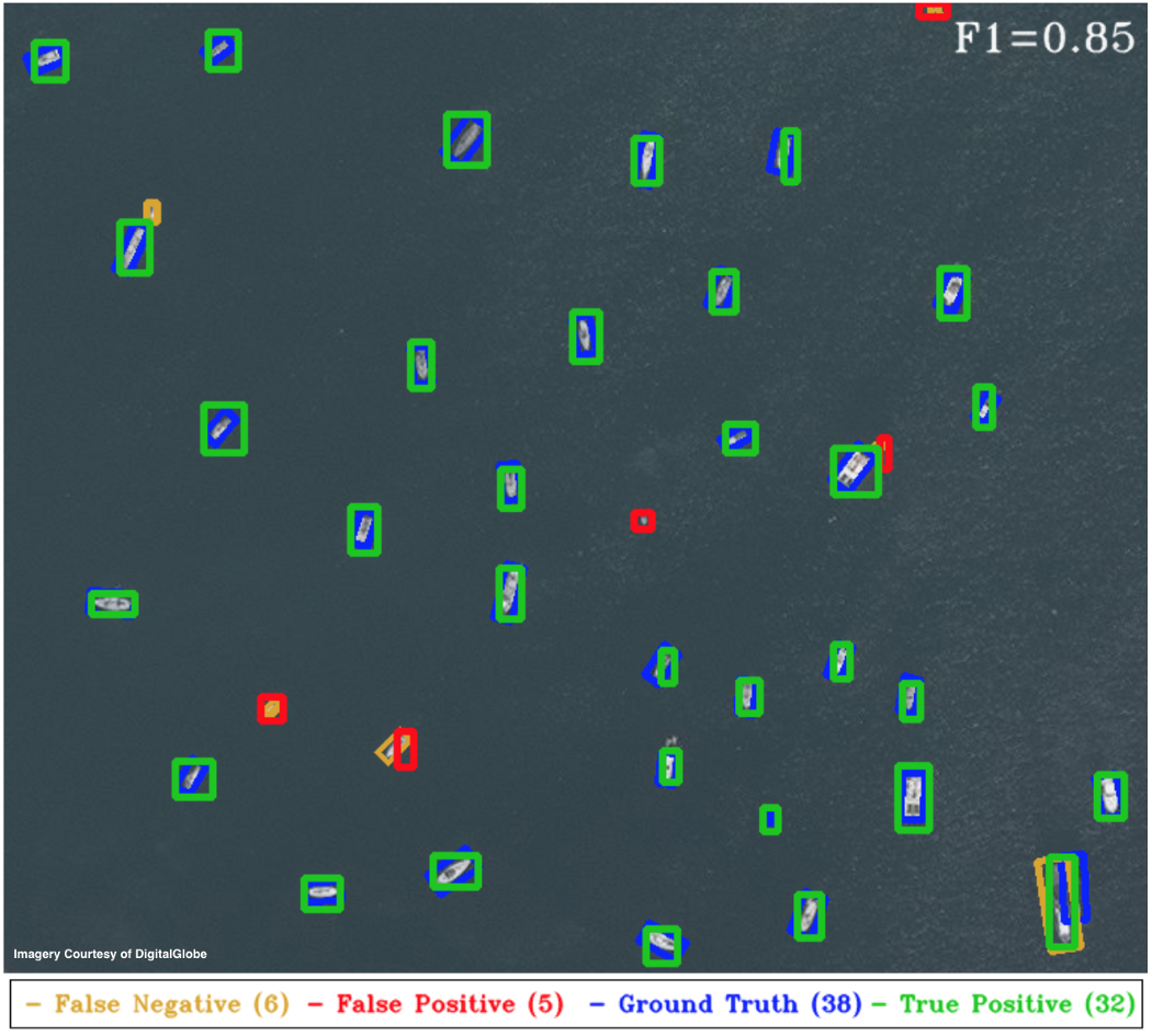
Figure 7. YOLT Performance on AOI2. As above, the incorrect detections are primarily due to incorrectly sized boxes for boats under 10m in length. Relaxing the Jaccard index threshold from 0.25 to 0.15 reduces the penalty on the smallest objects, and with this threshold the YOLT pipeline returns an F1 score of 0.93, comparable to the score of 0.96 achieved by the HOG + Sliding Window approach (see Figure 6 of 5).
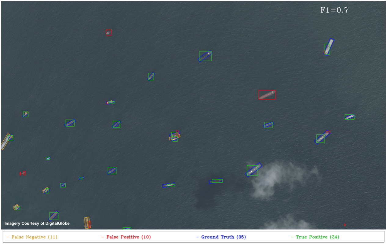
Figure 8. YOLT Performance on AOI3. The large false positive (red) in the right-center of the plot is an example of a labelling omission (error) which degrades our F1 score. Recall that for the HOG + Sliding Window approach the F1 score was 0.61 (see Figure 7 of 5).
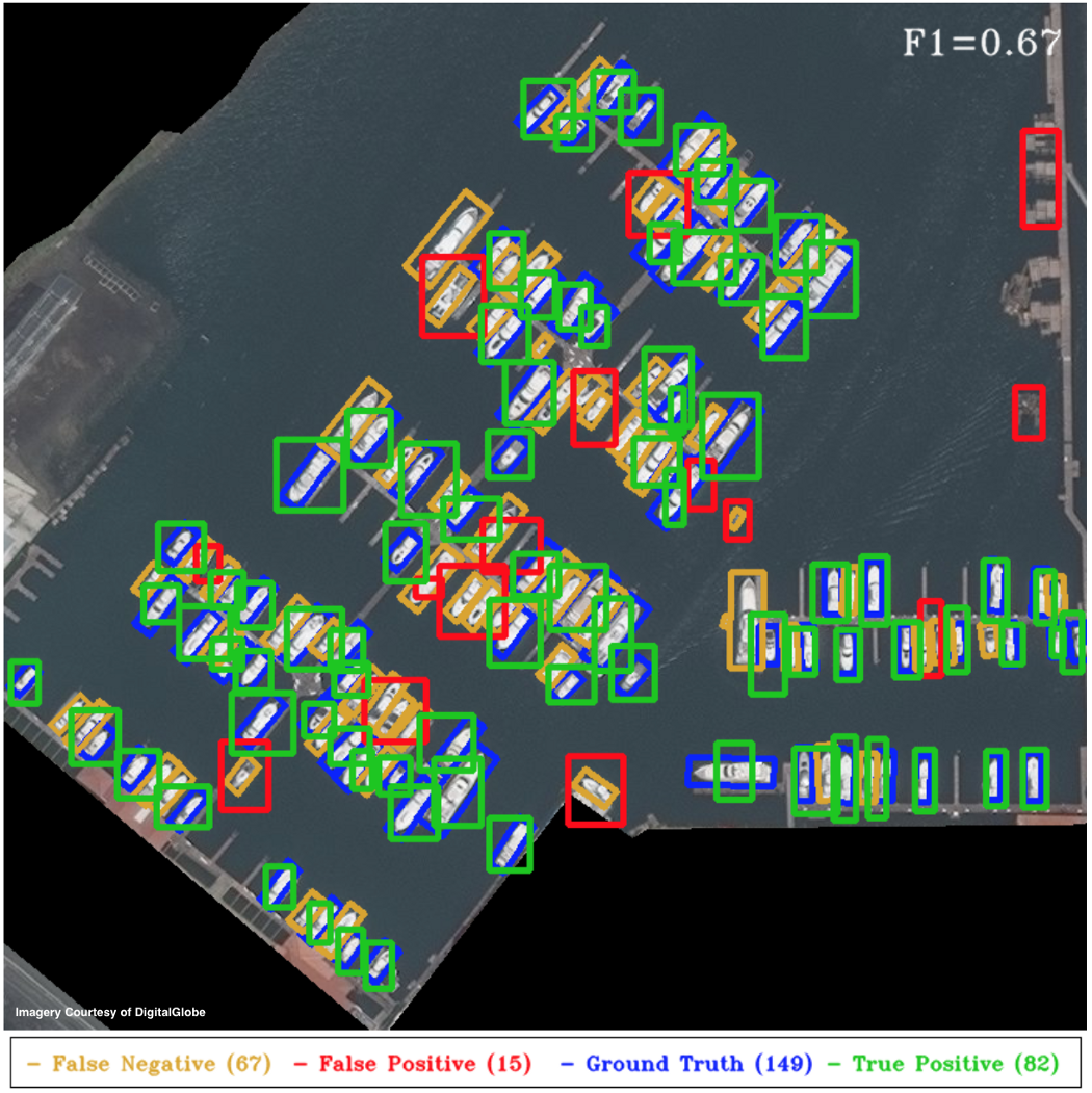
Figure 9. YOLT Performance on AOI4. The F1 score of 0.67 is not great, though it is actually better than the F1 of 0.57 returned by the naive implementation of HOG + Sliding Windows (see the inset of Figure 8 of 5). Incorporating rotated rectangular bounding boxes improved the score of Figure 8 of 5 from 0.57 to 0.86. Including heading information into the YOLT pipeline would require significant effort, though may be a worthwhile undertaking given the promise of this technique in crowded regions. Nevertheless, despite the modifications made to YOLO there may be a performance ceiling for densely clustered objects; a high-overlap sliding window approach can center objects at almost any location, so sliding windows combined with HOG (or other) features has inherent advantages in such locales.
각 이미지에 달린 설명이 굉장히 기네요. 그런데 하나씩 천천히 읽어보면 이해가 안 가는 내용은 아닙니다. 그냥 결과가 이렇다 설명하고 있는 파트입니다.
YOLT pipeline은 open water에서 잘 수행되지만, Figure 9를 보면 YOLO pipeline은 엄청나게 조밀한 영역에서는 차선책이 됩니다.
위에 나오는 4 areas는 모두 상대적으로 균일한 background를 갖고 있고, HOG + Sliding Window의 접근 방식이 잘 수행되는 지역입니다.

그러나 Figure 2에서 볼 수 있듯이, background가 매우 균일하지 않은 영역이라면 HOG + Sliding Window 접근 방식은 linear background features에서 boat의 차이를 찾는데 어려울 것입니다. Conv neural network는 이러한 scenes에서 가능성을 줍니다.
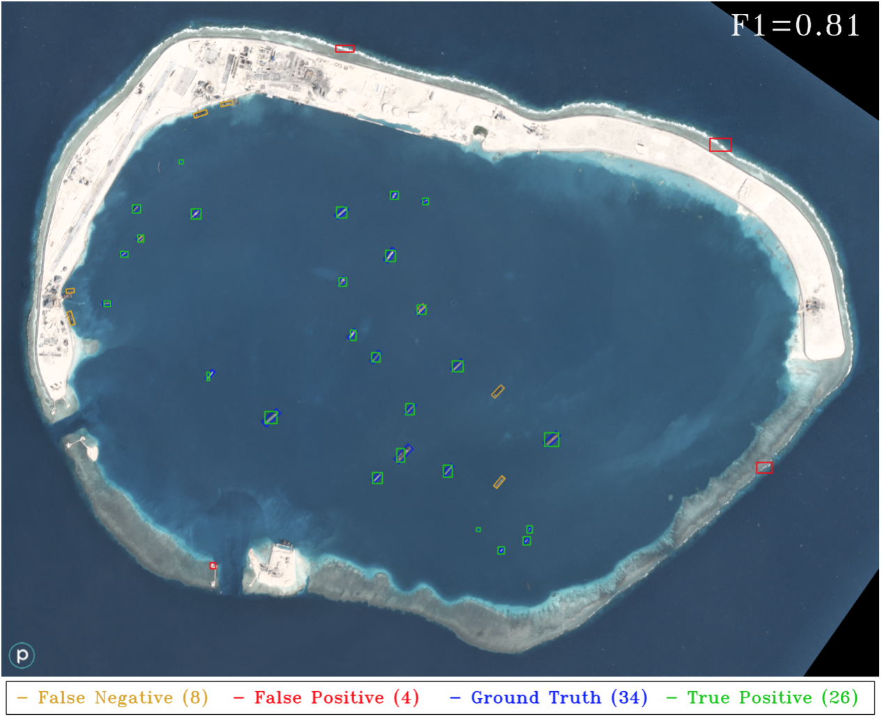
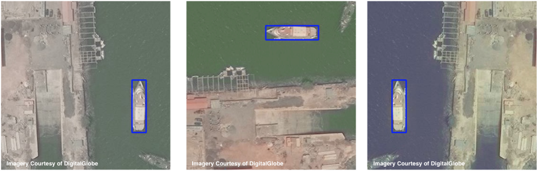
Figure 10. YOLT results for Mischief Reef using the same Planet test image as in Figure 2. Recall that only DigitalGlobe data is used for boat and airplane training. The classifier misses the docked boats, which is unsurprising since none of the training images contained boats docked adjacent to shore. Overall, the YOLT pipeline is far superior to the HOG + Sliding Window approach for this image, with ~20x fewer false positives and a nearly 3x increase in F1 score. This image demonstrates one of the strengths of a deep learning approach, namely the transferability of deep learning models to new domains. Running the YOLT pipeline on this image on a single GPU takes 19 seconds.
Figure 2와 Figure 10의 차이를 보시면 동일한 test image를 사용하여 YOLT한 결과가 Figure 10입니다. Figure 2의 classifier는 docked boats를 놓치는데, 해안에 근접해 있기 때문입니다.
전반적으로 YOLT pipeline이 이 이미지에 대한 HOG + Sliding Window 접근 방식보다 훨씬 더 우수하며 False Positive가 20배 이상 차이납니다. F1 Score도 3배 이상 증가합니다. 이 이미지는 딥러닝 모델을 새로운 영역으로 이전할 수 있음을 보여줍니다.
YOLT pipeline이 다른 data에서도 동일한 성능을 보여주는지 테스트하기 위해, 많은 boat가 있는 다른 이미지를 분석해봅니다.
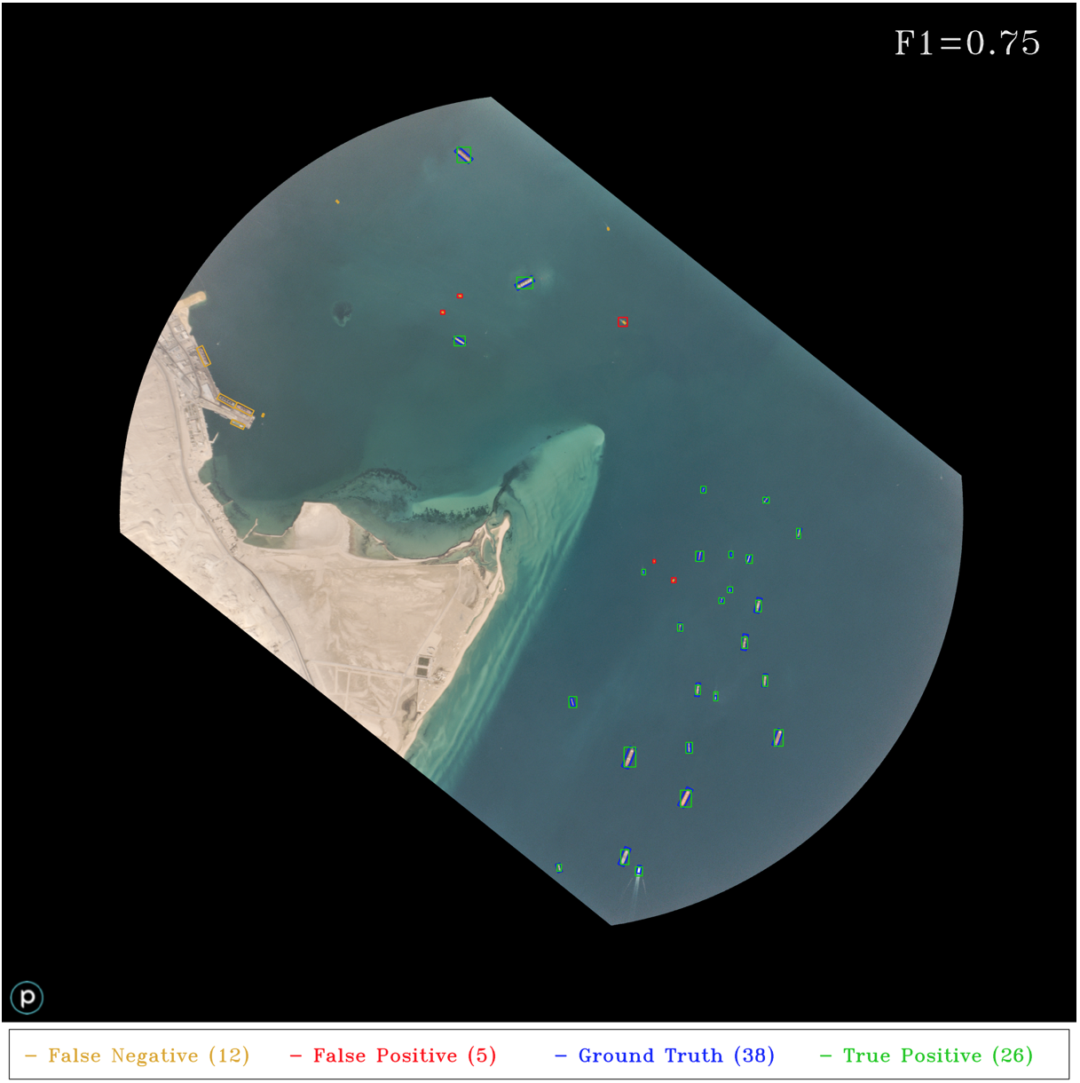
Figure 11. YOLT pipeline applied to a Planet image at the southern entrance to the Suez Canal. As in previous images, accuracy for boats in open water is very high. The only false negatives are either very small boats, or boats docked at piers (a situation poorly covered by training data). The five false positives are all actually located correctly, though the bounding boxes are incorrectly sized and therefore do not meet the Jaccard index threshold; further post-processing could likely remedy this situation.
해당 이미지에서도 accuracy는 굉장히 높습니다. False negative는 아주 작은 부둣가에 정박된 boat들이었습니다. Bbox의 크기가 잘못되어서 Jaccard Index 임게값을 충족하지 않지만 5개의 False Positive는 모두 실제로 올바르게 위치합니다. 이는 추가 후처리를 통해 해결 가능합니다.
마지막 테스트는 아래에서 볼 수 있듯이 classifier가 airplane에서 얼마나 잘 찾아내는지 확인합니다.
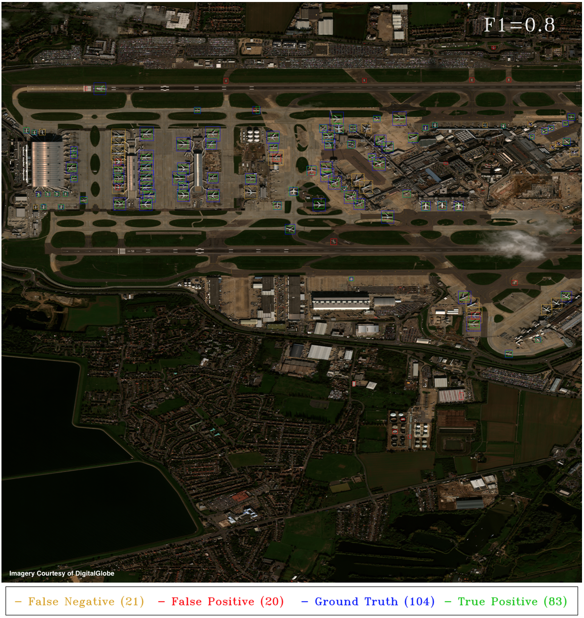
Figure 12. YOLT Detection pipeline applied to a DigitalGlobe image taken over Heathrow Airport. This is a complex scene, with industrial, residential, and aquatic background regions. The number of false positives is approximately equal to the number of false negatives, such that the total number of reported detections (103) is close to the true number of ground truth objects (104), though obviously not all positions are correct.
false positives랑 false negatives가 거의 같으므로 보고된 탐지의 수는 (103) 실제 ground truth object(104)와 가깝습니다!
6. Conclusion
이 게시글은 위성 영상의 object detection에 적용되는 machine learning techniques의 한계 중 하나인, background가 균일하지 않은 경우의 성능 저하되는 부분을 보여주었습니다.
이 한계를 해결하기 위해 위성 영상에서 boat, airplane 등을 빠르게 localize하기 위해 a fully convolutional neural network classifier (YOLT)를 구현했습니다.
이 classifier의 회전되지 않은 Bbox의 output은 매우 혼잡한 영역의 차선책이지만, sparse scenes에서는 HOG + Sliding Window 접근 방식보다 더 낫다는 것을 증명했습니다. 또한, 하나의 센서에서 훈련하고 다른 센서에서 모델을 적용하는 기능도 있었습니다.
논문 내용 첨부
You Only Look Twice: Rapid Multi-Scale Object Detection In
Satellite Imagery
방대한 양의 이미지에서 small object를 감지하는 것은 위성 영상의 주요 문제 중 하나입니다.
ground-based 이미지에서 object detection은 딥러닝 접근 방식에 대한 연구에 도움이 되었지만, 이 기술을 overhead image로 전환하는 것은 간단하지 않았습니다.
또한, 이미지 당 pixel 수와 지리적인 영역이었는데, 위성 영상은 엄청나게 많은 픽셀 값을 지닌다는 점이었습니다. 또한, 탐지하고자 하는 object가 매우 작아서(10 pixels 정도) 기존 CV 기술을 복잡하게 했습니다.
이 문제를 해결하기 위해 임의 크기의 위성 영상을 0.5 km^2 /s 의 속도로 평가하는 piplline(YOLT)를 제안했다. YOLT는 매우 빠르게 다른 object를 감지했고, 여러 센서에 대해 상대적으로 작은 training data로 확장됩니다.
기본 해상도(resolution)에서 large image를 evaluate하고 위치를 파악해 F1 Score 점수를 산출합니다. 점점 줄어드는 resolution에서 pipeline을 test하여 resolution 및 object size requirements를 추가 탐색합니다. 여기서는 5 pixels인 object도 여전히 높은 confidence로 localize할 수 있다는 결론을 내립니다!