타이타닉 데이터셋 분석

본 프로젝트는 멋쟁이사자처럼 AI School 6기 8팀이 함께 진행했습니다.

필요한 라이브러리 및 데이터 불러오기

import seaborn as sns
import pandas as pd
import numpy as np
import matplotlib.pyplot as plt

df = sns.load_dataset("titanic")

데이터셋 EDA 및 전처리

df.shape

(891, 15)

df.info()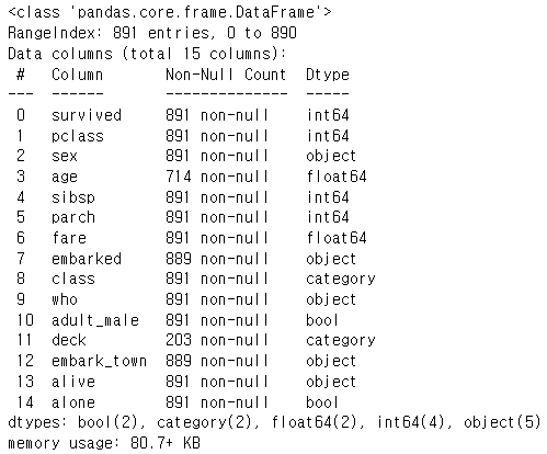

결측치 처리하기

• age랑 deck 변수안에 결측치가 꽤나 있는 것을 확인하였다. embark_town에도 조금 있는 것을 확인할 수 있었다.
• deck 이라는 변수안에는 결측치가 너무 많으므로 추후에 drop 시킨다.
• age의 경우 따로 나이를 설정해줄 수도 있으나 임의로 나이를 설정하기에는 결과에 영향을 많이 줄 것같으므로 나이에 결측치가 있는 행을 삭제해준다.
• embark_town의 경우도 위와 같이 실행한다.

df.isnull().sum()
# deck 이라는 변수 드랍 시키기
df=df.drop("deck", axis=1)
# 결측치가 들어있는 행 삭제 시키기
df=df.dropna()

필요없는 칼럼 삭제하기

메모리를 효율적으로 사용하기 위해

• alive와 survived는 같은 항목이므로 alive 칼럼을 drop
• sex와 who 칼럼으로 성인 남성이 이미 구분되므로 adult_male drop
  시킨다

df=df.drop('alive', axis=1)
df=df.drop('adult_male', axis=1)
df=df.drop("class", axis=1)

string으로 구성된 칼럼 변경하기

string 값으로 들어가 있는 칼럼들을 다음과 같이 바꿔준다.

def change_to_index(columns):
    tmp = {string : i for i,string in enumerate(df[columns].unique())}
    df[columns] = df[columns].map(tmp)
    print(tmp)

시각화를 통해 데이터 확인하기

• 결정 변수 안의 값 확인하기

df['survived'].value_counts()

• 전체 데이터에 대한 히스토그램 그려보기

_=df.hist(bins=50, figsize=(12,8))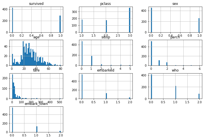

• 변수들간의 상관관계 분석하기
  가장 눈에 먼저 들어오는 것은 검정부분들인데,
  • (sex, survived)
  • (pclass, fare)
  • (sibsp, alone)
  • (parch, alone)
    를 대표적으로 뽑아 볼 수 있다.

_=sns.heatmap(data=df.corr())

의사결정나무

학습, 예측을 위한 사전 준비

# 종속변수 이름 설정하기
label_name='survived'

# 독립변수 이름 리스트 설정하기
feature_names=df.columns.tolist()
feature_names.remove(label_name)
feature_names

# 각 X와 y 만들어주기
X=df[feature_names]
y=df[label_name]
X.shape, y.shape

training과 test 데이터셋 만들기

from sklearn.model_selection import train_test_split
from sklearn.tree import DecisionTreeClassifier
from sklearn.tree import plot_tree
from sklearn.metrics import accuracy_score
from sklearn.model_selection import cross_val_predict
from sklearn.model_selection import GridSearchCV
from sklearn.model_selection import RandomizedSearchCV

X_train, X_test, y_train, y_test = train_test_split(X,
                                                   y,
                                                   test_size=0.2,
                                                   stratify=y,
                                                   random_state=42)

의사결정나무 모델 구축하기(하이퍼 파라미터 튜닝X)

우선 하이퍼파라미터 따로 튜닝 하지 않고,
* max_depth=15
* max_features=0.9
* random_state=42  
를 이용하여 의사결정나무 모델을 구축해보도록 하겠다

알고리즘 가져오기

model = DecisionTreeClassifier(max_depth=10, 
                               max_features=0.9, 
                               random_state=42)

학습시키기

model.fit(X_train, y_train)

y_predict = model.predict(X_test)

plt.figure(figsize=(20, 20))
plot_tree(model, filled=True, fontsize=14, feature_names=feature_names)
plt.show()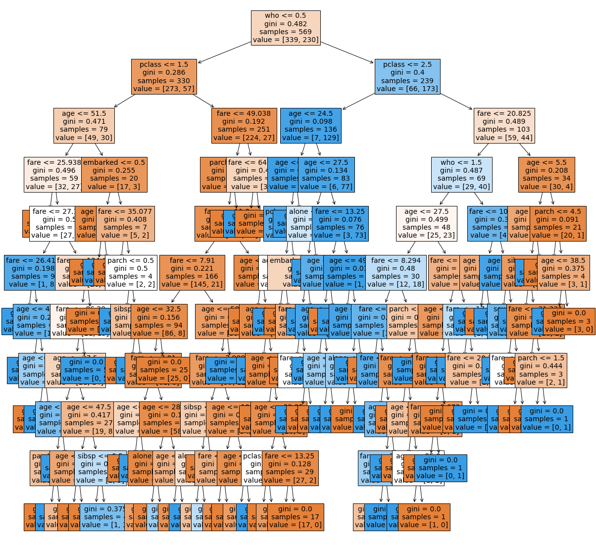

Feature 중요도 확인하기

sns.barplot(x=model.feature_importances_, y=feature_names)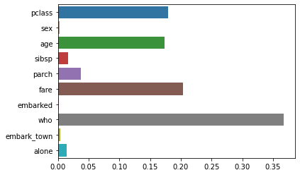

위의 결과를 통해 who의 중요도가 가장 높게 나왔고, embark_town의 중요도가 가장 낮은 것으로 나오는것을 확인할 수 있었다.

정확도 측정하기

accuracy_score(y_test, y_predict)

0.7132867132867133

정확도는 대략 78% 정도가 나왔음을 확인할 수 있다.

의사결정나무 모델 구축하기(GridSearchCV)

# 각 파라미터에 대한 리스트를 만들어주기
max_depth_list = [2,3,5,7,9,12,15,20,40]
max_features_list =[0.1,0.2, 0.3,0.4,0.5,0.6,0.7,0.8,0.9,1]

학습시키기

#GridSearchCV에 적용하기
parameters = {'max_depth':max_depth_list, 'max_features':max_features_list}

clf=GridSearchCV(model, param_grid=parameters, scoring="accuracy", n_jobs=-1, cv=5)
clf.fit(X_train,y_train)

• GridSearchCV를 이용하여 모델을 돌려본 결과 다음과 같은 파라미터에서 다음과 같은결과가 가장 높은 결과라는 것을 알 수 있었다.
• 확실히 파라미터를 임의로 선택하였을 때보다 더 높은 정확도를 보인다는 것을 확인할 수 있다.

clf.best_estimator_

DecisionTreeClassifier(max_depth=3, max_features=0.7, random_state=42)

clf.best_score_

0.8382394038192829

Feature 중요도 확인하기
who의 중요도가 더 상승하였고, pclass, age, fare 순으로 중요도를 가지고 있음을 확인할 수 있었다.

best_model_grid=clf.best_estimator_
best_model_grid.fit(X_train,y_train)

sns.barplot(x=best_model_grid.feature_importances_,y=feature_names)

의사결정나무 모델 구축하기(RandomSearchCV)

max_depth_list = [2,3,5,7,9,12,15,20,40]
max_features_list =[0.1,0.2, 0.3,0.4,0.5,0.6,0.7,0.8,0.9,1]

학습시키기

param_distributions={"max_depth": max_depth_list, "max_features":max_features_list }

clf=RandomizedSearchCV(model, param_distributions,cv=5,n_jobs=-1,random_state=42,n_iter=5)

clf.fit(X_train,y_train)

같은 조건에서

• RandSearchCV를 이용하여 max_depth=5, max_features=0.3 일때 가장 좋은 결과를 얻을 수 있었다.
• GridSearchCV를 이용하였을 때보단 정확도는 더 떨어진 모습을 보이고 있다.

clf.best_estimator_

DecisionTreeClassifier(max_depth=5, max_features=0.3, random_state=42)

clf.best_score_

0.8137401024685609

Feature 중요도 확인하기
위와 같이 who의 중요도가 가장 높았고 pclass, age, fare 순으로 중요도가 높았다

best_model_rand=clf.best_estimator_
best_model_rand.fit(X_train,y_train)

DecisionTreeClassifier(max_depth=5, max_features=0.3, random_state=42)

sns.barplot(x=best_model_rand.feature_importances_,y=feature_names)

의사결정나무 모델 구축하기(GridSearchCV, RandSearchCV)

max_feature을 np.random으로 파라미터 리스트 만들어서 진행하기

max_depth_list=[i for i in range(1,11)]
max_features_list=np.random.uniform(0.3,0.9,20)

함수로 만들어서 한번에 비교하기
매번 넣어주는 리스트의 구성마다 매번 다를 거기 때문에 함수로 만들어서 진행하기

def compare_GR(depth,feature):
    #gridsearch
    import time
    start = time.time()
    parameters = {'max_depth':max_depth_list, 'max_features':max_features_list}
    clf=GridSearchCV(model, param_grid=parameters, scoring="accuracy", n_jobs=-1, cv=5)
    clf.fit(X_train,y_train)
    grid_score=clf.best_score_
    print(f'GridSearch\n')
    print(f'Best Score parameters: {clf.best_estimator_}\n')
    print(f'Best Score: {grid_score}\n')
    print(f'Time: {time.time() - start}\n')
    print('-------------------------------------------------------------\n')
    
    
    #randsearch
    start = time.time()
    param_distributions={"max_depth": max_depth_list, "max_features":max_features_list }
    clf=RandomizedSearchCV(model, param_distributions,cv=5,n_jobs=-1,random_state=42,n_iter=5)
    clf.fit(X_train,y_train)
    rand_score=clf.best_score_
    print(f'RandSearch\n')
    print(f'Best Score parameters: {clf.best_estimator_}\n')
    print(f'Best Score: {rand_score}\n')
    print(f'Time: {time.time() - start}\n')
    print('-------------------------------------------------------------\n')
    
    #비교하기
    if grid_score > rand_score:
        print('GridSearhcv의 정확도가 더 높습니다.')
    elif grid_score < rand_score:
        print('RandSearhcv의 정확도가 더 높습니다.')
    elif grid_score==rand_score:
        print('같습니다')
    else:
        print('뭔가 이상합니다')

결론

compare_GR(max_depth_list,max_features_list)

GridSearch

Best Score parameters: DecisionTreeClassifier(max_depth=3, max_features=0.7513902397624934,
random_state=42)

Best Score: 0.8382394038192829

Time: 0.8767976760864258

---

RandSearch

Best Score parameters: DecisionTreeClassifier(max_depth=5, max_features=0.39089207858316505,
random_state=42)

Best Score: 0.8137401024685609

Time: 0.04804348945617676

---

GridSearhcv의 정확도가 더 높습니다.