따릉이 데이터 분석하기 (5) Tree

따릉이 데이터 분석하기 (5) Tree

이번에는 Tree 관련 모델들로 주어진 데이터셋을 훈련시켜보고 이를 검증해보도록 하자. 저번 Transformation 데이터 분석 과정과 마찬가지로 scikit-learn의 Pipeline을 이용해 데이터 전처리부터 모델링까지의 파이프라인을 구성해보도록 하겠다. Data Load와 Preprocessing 관련 코드 및 자세한 설명은 시리즈의 이전 게시글을 참고하면 될 것이다.

Decision Tree Regressor

우선 다음 구조와 같은 가장 간단한 형태의 Tree Regressor을 만들어보도록 하자.

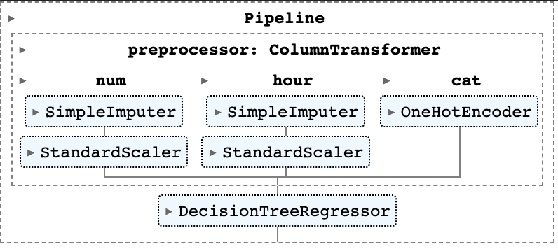
이전과 마찬가지로 Pipeline 모듈을 이용해 모델을 구성했다. 코드는 다음과 같다.

# Tree Regressor
from sklearn.tree import DecisionTreeRegressor
tree_reg = Pipeline(
    steps=[("preprocessor",preprocessor),
    ("tree",DecisionTreeRegressor(criterion="squared_error"))]
)
tree_reg.fit(X_train, y_train)

여기서는 Tree Regression 과정의 criterion으로 제곱오차를 지정한 것 외에는 별다른 하이퍼파라미터를 지정하지 않았다. 따라서 어떤 형태로 모델이 형성되었는지 살펴보면, 아래와 같이 tree의 깊이(depth)가 20이고 총 leave(트리의 잎 노드 : 자식 노드가 없는 노드를 의미함)의 개수는 967개인 것을 확인할 수 있다. 또한, 위 모델로 Validation data에 대해 RMSE를 계산해 보면 50.643의 값을 얻을 수 있다.

# Tree Info and Validation RMSE
tree_res = tree_reg.named_steps['tree']
tree_res.get_depth() # 20
tree_res.get_n_leaves() # 967
tree_pred = tree_reg.predict(X_val)
np.sqrt(mean_squared_error(y_val, tree_pred)).round(3) # 50.643

GridSearch

하지만, 개별 트리를 만드는 데에도 앞서 언급한 트리의 깊이, 잎 노드의 개수 등을 포함한 많은 하이퍼파라미터가 요구된다. 적당한 하이퍼파라미터를 찾기 위해 GridSearch를 이용해 찾아보도록 하자. Scikit-learn 패키지는 GridSearchCV라는 cross-validation과 Grid serach를 동시에 진행하는 알고리즘을 갖고 있으나, 여기서는 이미 주어진 validation 데이터를 활용하기 위해 GridSearch만 진행하는 알고리즘을 직접 코딩했다. 코드는 아래와 같다.

# Check whether Overfitted with Cross-Validation
from tqdm import * # Progress-bar
from sklearn.model_selection import GridSearchCV
params = {'max_features':("sqrt","log2","auto"), "max_depth" : list(range(2, 41, 2))}

# GridSearch Algorithm
N_comb = len(params['max_features']) * len(params['max_depth'])
with tqdm(total=N_comb) as pbar:
    df = []
    for feat in params['max_features']:
        scores = []
        for d in params['max_depth']:
            reg_i = Pipeline(
                steps=[('preprocessor',preprocessor),('tree',DecisionTreeRegressor(max_features=feat,max_depth=d))]
            )
            reg_i.fit(X_train,y_train)
            pred_i = reg_i.predict(X_val)
            score_i = np.sqrt(mean_squared_error(y_val, pred_i)).round(3)
            scores.append(score_i)
            pbar.update()
        df.append(scores)
res = pd.DataFrame(df, index=params['max_features'], columns=params['max_depth']).T

GridSearch는 하이퍼파라미터 max_features와 max_depth에 대해서만 진행했다. 이는 각각 split 단계에서 몇 개의 feature을 랜덤으로 추출해 best splitting variable을 찾을 것인지와, 트리의 깊이를 최대 어느정도로 설정할 것인지를 의미한다. 위 코드를 실행하면 결과로 데이터프레임 res를 얻는데, 이는 각 hyperparmeter 조합(총 $3\times20=60$)에 대한 Validation RMSE 값을 포함한다. 이를 Plot으로 나타내면 다음과 같다(코드는 Github 참고).

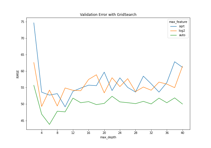
이를 확인해보면 모두 max_depth가 4,6,8,10 등 낮은 값에서 Validation RMSE가 낮은 것을 확인할 수 있으며, max_feature의 경우 auto(각 단계에서 모든 변수를 고려함)가 다른 두 기준보다(sqrt : 각 단계에서 $\sqrt p$ 만큼 고려, log2 : $\log_2 p$ 만큼 고려) 더 나은 지표를 보이는 것을 확인할 수 있다.

Tree with PCA

이번에는 트리 모델 이전에 PCA를 적용시켜 차원 축소를 바탕으로 더 나은 성과를 낼 수 있는지 확인해보도록 하자. 코드는 아래와 같은데, 우선 각 인덱스 idx는 각 max_features에 대해 가장 낮은 RMSE를 갖는(최적의) max_depth 파라미터 값을 의미한다. 즉 idx_1의 경우 "auto" 모델을 최소로 하는 max_depth=6의 값이 될 것이다. 이를 바탕으로 PCA를 포함한 Pipeline을 만들었는데, 여기서 n_components=3을 선택한 이유는 이전 Transformation 글에서 확인할 수 있다. 이를 바탕으로 각 모델이 데이터들을 어떻게 fitting하는지 살펴보도록 하자. 이를 위해 Validation 데이터들을 첫번째 주성분(principal component)으로 projection한 후, 이들을 순서대로 정렬해 predict value에 대한 Line plot을 그려보도록 하자. 코드는 다음과 같다.

# Three Models : For each max_feature, the argmin max_depth
idx_1 = res.index[np.argmin(res['auto'])]
idx_2 = res.index[np.argmin(res['log2'])]
idx_3 = res.index[np.argmin(res['sqrt'])]


tree_pca_1 = Pipeline(
    steps=[('preprocessor',preprocessor),
        ('pca', PCA(n_components=3)),
        ('tree',DecisionTreeRegressor(max_features='auto',max_depth=idx_1))]
)
tree_pca_2 = Pipeline(
    steps=[('preprocessor',preprocessor),
        ('pca', PCA(n_components=3)),
        ('tree',DecisionTreeRegressor(max_features='log2',max_depth=idx_2))]
)
tree_pca_3 = Pipeline(
    steps=[('preprocessor',preprocessor),
        ('pca', PCA(n_components=3)),
        ('tree',DecisionTreeRegressor(max_features='sqrt',max_depth=idx_3))]
)
tree_pca_1.fit(X_train, y_train)
tree_pca_2.fit(X_train, y_train)
tree_pca_3.fit(X_train, y_train)

pca = tree_pca_1[0:2] # Pipeline until PCA
xs_1, ys_1 = zip(*sorted(zip(pca.transform(X_val)[:,0],tree_pca_1.predict(X_val))))
xs_2, ys_2 = zip(*sorted(zip(pca.transform(X_val)[:,0],tree_pca_2.predict(X_val))))
xs_3, ys_3 = zip(*sorted(zip(pca.transform(X_val)[:,0],tree_pca_3.predict(X_val))))

# Compare three Local_Minimum RMSE spot
# Projeted on the first Principal Component

# Plot
fig, axes = plt.subplots(3,1,figsize=(10,15), constrained_layout=True)
axes[0].scatter(pca.transform(X_val)[:,0], y_val, alpha=0.4, label='data')
axes[0].plot(xs_1, ys_1, label = 'max_feature = "auto"', color = "darkgreen", linewidth = 2)
axes[0].legend(fontsize = 12, loc = 'upper right')
axes[0].set(xlabel = "First Principal Component", ylabel="Y",title=f"Tree with PCA : max_depth = {idx_1}")

axes[1].scatter(pca.transform(X_val)[:,0], y_val, alpha=0.4, label='data')
axes[1].plot(xs_2, ys_2, label = 'max_feature = "log2"', color = "orange", linewidth = 2)
axes[1].legend(fontsize = 12, loc = 'upper right')
axes[1].set(xlabel = "First Principal Component", ylabel="Y",title=f"Tree with PCA : max_depth = {idx_2}")

axes[2].scatter(pca.transform(X_val)[:,0], y_val, alpha=0.4, label='data')
axes[2].plot(xs_3, ys_3, label = 'max_feature = "sqrt"', color = "navy", linewidth = 2)
axes[2].legend(fontsize = 12, loc = 'upper right')
axes[2].set(xlabel = "First Principal Component", ylabel="Y",title=f"Tree with PCA : max_depth = {idx_3}")


plt.savefig("plots/tree_pca.png", transparent=False, facecolor='white')

위 코드를 실행하면 다음과 같은 세 개의 plot을 얻을 수 있다.

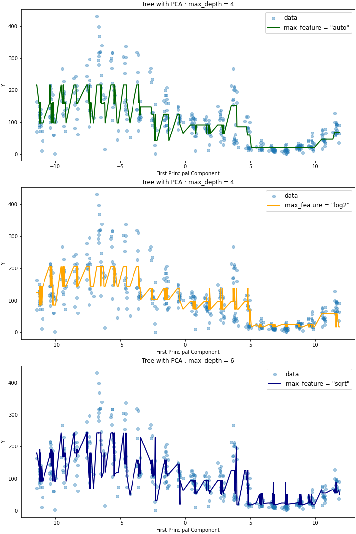
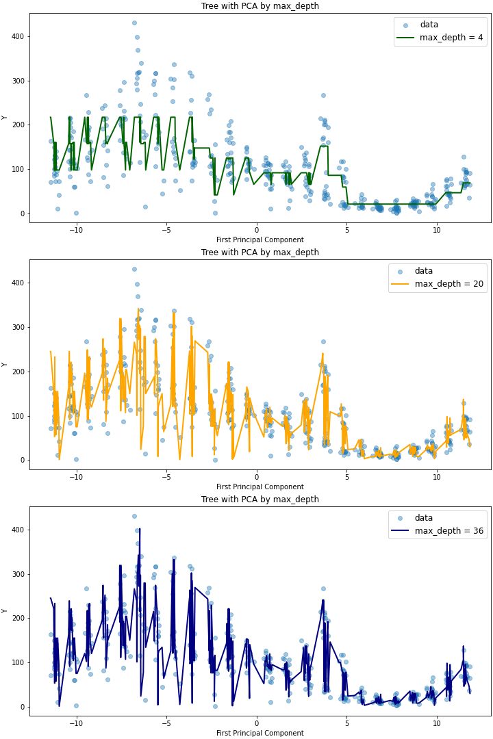
이를 살펴보면 max_depth가 같지만 max_features가 다른 auto,log2 모델에 대해서는 plot의 적합도가 유사하지만, max_depth=6으로 트리의 깊이가 더 깊은 sqrt 모델에 대해서는 더 outlying한 데이터에 대해서도 예측이 잘 이루어지는 것을 확인할 수 있다. max_features를 동일하게 두고(auto) 트리의 깊이에 따른 영향을 확인해보면 다음과 같은데(코드는 Github 참고), max_depth가 20인 경우와 36인 경우 RMSE가 유사한 것과 마찬가지로 모델 역시, 더 outlying한 데이터를 36일 때 잘 캐치한다는 것 외에는 전체적으로 유사함을 확인할 수 있다.

Gradient Boosted Decision Trees

이번에는 GBM을 이용한 Decision Tree Regression 모델(Gradient Boosted Decision Trees, 이하 GBDT)을 살펴보도록 하자. scikit-learn의 sklearn.ensemble 모듈 에서는 Regression에 사용가능한 GBDT 모델 GradientBoostingRegressor 을 제공하고 있다. 이를 이용하여 이번에는 scikit-learn의 자체 gridsearch module인 sklearn.model_selection.GridSearchCV으로 하이퍼파라미터 최적화를 진행해보도록 하겠다. 이때, GridSearchCV를 사용하기 위해 Validation scoring을 위한 기준이 필요한데, 여기서는 RMSE를 사용할 것이므로 이를 별도로 정의해주는 과정이 필요하다. 코드는 다음과 같다.

# GBDT with GridsearchCV
from sklearn.ensemble import GradientBoostingRegressor
from sklearn.model_selection import GridSearchCV
from sklearn.metrics import make_scorer

# RMSE def for Gridsearch Scoring
def rmse(y_true, y_pred):
    mse = mean_squared_error(y_true, y_pred)
    return(np.sqrt(mse))
rmse_score = make_scorer(rmse, greater_is_better=False)
# Pipeline Model
tree_gbm = Pipeline([
("preprocessor",preprocessor),("gbm",GradientBoostingRegressor(loss='squared_error',max_features='auto'))
])

위와 같이 scoring 객체를 만들고 GBDT의 파이프라인을 만들면, 아래와 같이 parameter grid를 정의하여 GridSearch를 진행할 수 있다.

# Gridsearch
param_grid = {
    'gbm__n_estimators' : 10 * np.logspace(base=2, start=0, stop=5, num=6).astype(int),
    'gbm__max_depth' : np.linspace(4,32,8).astype(int)
}
search = GridSearchCV(
    tree_gbm, param_grid, verbose = 5, n_jobs= 5, scoring = rmse_score
)
search.fit(X_train, y_train)

이전과는 다르게, gridsearch parameter로 max_feature 대신 n_estimators를 이용했다. 이는 Boosting 단계가 몇번 반복될지를 정의하는 것으로, 일반적으로 Gradient boosting 방식은 과적합에 robust하므로 큰 값이 더 좋은 결과를 가지는 경향이 있다. fitting을 진행하게 되면, search.cv_results_로 파라미터 조합 별(총 240개) fit/score time(훈련 및 테스트 시간), 각 split별 score(여기서는 기본인 5-folds validation 이므로 총 5개 값)들과 평균, 표준편차를 딕셔너리 형태로 얻어 이를 데이터프레임으로 변환할 수 있다(아래 표 참고).

mean_fit_time	std_fit_time	mean_score_time	std_score_time	param_gbm__max_depth	param_gbm__n_estimators	params	split0_test_score	split1_test_score	split2_test_score	split3_test_score	split4_test_score	mean_test_score	std_test_score	rank_test_score
0.249	0.063	0.061	0.016	4	10	{'gbmmax_depth': 4, 'gbmn_estimators': 10}	-53.869	-45.526	-53.144	-51.671	-48.405	-50.523	3.125	17

✅참고로, GridSearch 방식은 일반적인 노트북 환경에서는 훈련 시간이 상당히 많이 소요되기 때문에 나의 경우 Google Colab을 이용했고, Colab에서 얻은 search.cv_results_ 데이터프레임을 별도의 로그로 저장해 다시 로컬에서 불러오는 방법을 이용했다.

Plot for GBDT Gridsearch

이렇게 얻은 GridSearch 결과를 이용해 파라미터 조합 별 Mean test score을 아래와 같이 plot으로 나타내보도록 하자. (코드 참고 : https://stackoverflow.com/questions/37161563/how-to-graph-grid-scores-from-gridsearchcv - 오류가 있어 일부 코드 수정함)

# Plot search_res
def plot_grid_search(cv_results, grid_param_1, grid_param_2, name_param_1, name_param_2, greater_is_better):
    # Get Test Scores Mean and std for each grid search
    if greater_is_better: 
        scores_mean = cv_results['mean_test_score']
    else: # greater_is_better = False면 score 값이 음수임
        scores_mean = -cv_results['mean_test_score']

    scores_mean = np.array(scores_mean).reshape(len(grid_param_1),len(grid_param_2))

    # Plot Grid search scores
    fig, ax = plt.subplots(1,1, figsize = (10,10))

    # Param1 is the X-axis, Param 2 is represented as a different curve (color line)
    for idx, val in enumerate(grid_param_2):
        ax.plot(grid_param_1, scores_mean[:,idx], '-o', label= name_param_2 + ': ' + str(val))

    ax.set_title("Grid Search Scores", fontsize=15, fontweight='bold')
    ax.set_xlabel(name_param_1, fontsize=12)
    ax.set_ylabel('CV Average Score', fontsize=12)
    ax.legend(loc="best", fontsize=12)
    ax.grid('on')
    plt.savefig('plots/tree_gbm_gridsearchcv.png', facecolor='white', transparent=False)

plot_grid_search(search_res, 
    param_grid['gbm__max_depth'],
    param_grid['gbm__n_estimators'],
    'max_depth', 'n_estimators', greater_is_better=False)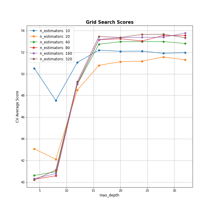

Validation

이제 search.best_params_를 통해 GridSearch에서 얻은 최적의 하이퍼파라미터 조합을 얻을 수 있지만, 로컬에는 fit model이 저장되어있지 않으므로 앞서 얻은 result dataframe에 저장되어있는 ranking으로 쉽게 구할 수 있다. best hyperparmeter인 max_depth = 4, n_estimators = 320을 이용하여 train_test_split 으로 처음에 구한 Validation data에 대해 RMSE를 구하면 다음과 같다.

# Best_params
best_params = search_res.loc[search_res['rank_test_score']==1,["param_gbm__max_depth","param_gbm__n_estimators"]]
gbdt_best = Pipeline([
("preprocessor",preprocessor),
("gbm",GradientBoostingRegressor(
    loss='squared_error',max_features='auto',
    max_depth=best_params.iloc[0,0], n_estimators=best_params.iloc[0,1]))
])
gbdt_best.fit(X_train,y_train)
rmse(y_true=y_val, y_pred=gbdt_best.predict(X_val)) # 36.827

오히려 Cross validation error보다 더 낮은 RMSE가 도출되는 것을 확인할 수 있다.

Random Forest

이제 마지막으로 트리 활용 모델 중 가장 인기(?)있다고 할 수 있는 랜덤포레스트 모델을 구현해보도록 하자. 랜덤포레스트 모델도 마찬가지로 튜닝해야할 Hyperparmeter가 존재하기 때문에, 적절한 hyperparameter을 선택하여 Gridsearch를 진행해보도록 하겠다(Colab 이용). 총 네 개의 hyperparmeter n_estimators(랜덤포레스트당 개별 트리의 개수), max_features, max_depth, min_samples_split(한 노드를 split하기 위해 필요한 최소한의 샘플 개수) 에 대해 적당한 값을 Grid로 취하여 훈련을 진행했다.

# RandomForest Regressor
from sklearn.ensemble import RandomForestRegressor
rf_reg = Pipeline(steps=[('preprocessor',preprocessor),('rf',RandomForestRegressor())])
param_grid = {
    'rf__n_estimators' : [50, 100, 200, 400], # number of trees
    'rf__max_features' : ['auto','sqrt'],
    'rf__max_depth' : [5, 10, 15, 20],
    'rf__min_samples_split' : [2, 6, 10],
    'rf__bootstrap' : [True]
}
reg = GridSearchCV(rf_reg, param_grid, verbose=10, scoring=rmse_score)
reg.fit(X_train, y_train)

이를 바탕으로 최선의 하이퍼파라미터 조합 best_params를 다음과 같이 선택한 후, 이를 이용해 랜덤포레스트 파이프라인을 재구성했다.

# Return best parameter of Gridsearch at RandomForest
rf_res = pd.read_csv('logs/rf_grid_res.csv',index_col=0)
best_params = rf_res.loc[rf_res.rank_test_score==1,[i for i in rf_res.columns if 'param_' in i]]
n_params = []
for i in best_params.columns:
    n_params.append(i[10:])
best_params.columns = n_params
best_params = best_params.to_dict('records')[0]
# RF with best params
rf_best= Pipeline(steps=[('preprocessor',preprocessor),('rf',RandomForestRegressor(**best_params))]) # ** as kwargs unpacking
rf_best.fit(X_train, y_train)

또한, 랜덤포레스트 모델의 특징으로 회귀분석처럼 변수의 중요도를 특정 기준에 의해 측정할 수 있는데, 다음과 같이 Pipeline의 randomforest 모형에서의 attribute rfreg.feature_importances_로 그 결과를 얻을 수 있고, 이를 bar chart로 간단히 표현해보았다.

# Variable Importance
rfreg = rf_best.named_steps['rf']
idx= list(X_train.columns.drop('precip'))
idx.extend(['precip_0','precip_1'])
importance = pd.DataFrame(rfreg.feature_importances_[:-1], idx).round(3)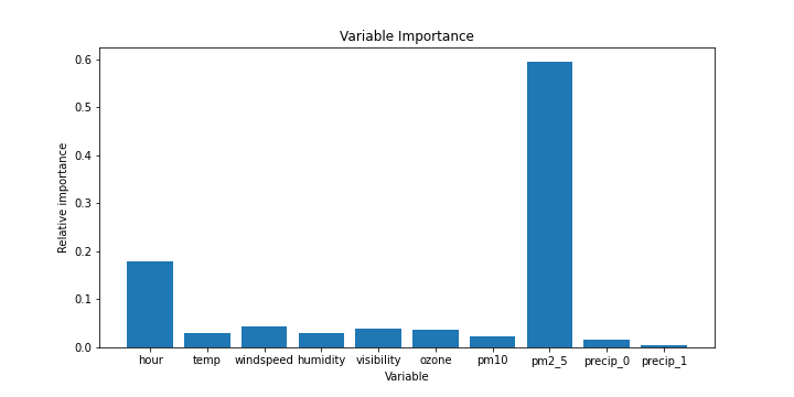

마지막으로, 랜덤포레스트 모형에 대해서도 Validation data에 대한 RMSE를 구해본 결과 다음과 같이 꽤 괜찮은 값을 얻을 수 있었다.

# Validation
pred_rf = rf_best.predict(X_val)
rmse(y_val, pred_rf) # 35.882

• 🖥 Full code on Github : https://github.com/ddangchani/project_ddareungi