[TIL Day25] E2E 머신러닝 프로젝트

이다혜·2021년 6월 3일

project

TIL

목록 보기

26/60

End-to-End 머신러닝 프로젝트

부동산 회사에 막 고용된 데이터 과학자라고 가정하고 예제 프로젝트를 진행해보자. 주요 단계는 다음과 같다. 캘리포니아 주택 가격 데이터셋을 사용한다. Original Code

Look at the big picture.
Get the data.
Discover and visualize the data to gain insights.
Prepare the data for Machine Learning algorithms.
Select a model and train it.
Fine-tune your model.
Present your solution.
Launch, monitor, and maintain your system.

1. 큰 그림 보기

모델이 전체 시스템 안에서 어떻게 사용될 지를 이해하는 것이 중요하다.

풀어야 할 문제: 캘리포니아 인구조사 데이터를 사용해 캘리포니아의 주택 가격 모델을 만드는 것
중요한 질문: 현재 솔루션은? 전문가가 수동으로? 복잡한 규칙? 머신러닝?

문제 정의

지도학습, 비지도학습, 강화학습 중에 어떤 경우에 해당하는가?
분류문제인가, 아니면 회귀문제인가?
배치학습(=오프라인학습), 온라인학습(=점진적학습) 중 어떤 것을 사용해야 하는가? 차이점은 여기참고!

성능측정지표(performance measure) 선택

평균제곱근 오차(root mean square error (RMSE))
$\mathrm{RMSE}(\mathbf{X}, h) = \sqrt{\frac{1}{m}\sum_{i=1}^{m}\left(h\left(\mathbf{x}^{(i)}\right)-y^{(i)}\right)^2}$
- $m$ : 데이터셋에 있는 샘플 수
- $\mathbf{x}^{(i)}$ : $i$ 번째 샘플의 전체 특성값의 벡터(vector)
- $y^{(i)}$ : $i$ 번째 샘플의 label(해당 샘플의 기대 출력값)
- $\mathbf{X}$ : 데이터셋 모든 샘플의 모든 특성값(features)을 포함하는 행렬(matrix)
- $h$ : 예측함수(prediction function). 하나의 샘플 $\mathbf{x}^{(i)}$ 에 대해 예측값 $\hat{y}^{(i)} = h\left(\mathbf{x}^{(i)}\right)$ 를 출력함.

2. 데이터 가져오기

import os
import tarfile
import urllib

DOWNLOAD_ROOT = "https://raw.githubusercontent.com/ageron/handson-ml2/master/"
HOUSING_PATH = os.path.join("datasets", "housing")
HOUSING_URL = DOWNLOAD_ROOT + "datasets/housing/housing.tgz"


def fetch_housing_data(housing_url=HOUSING_URL, housing_path=HOUSING_PATH):
    if not os.path.isdir(housing_path):
        os.makedirs(housing_path)
    tgz_path = os.path.join(housing_path, "housing.tgz")
    urllib.request.urlretrieve(housing_url, tgz_path)
    housing_tgz = tarfile.open(tgz_path)
    housing_tgz.extractall(path=housing_path)
    housing_tgz.close()
    
# fetch_housing_data를 호출하면 현재 작업공간에 datasets/housing 디렉토리를 만들고 
# housing.tgz 파일을 내려받고 압축을 풀어 housing.csv 파일을 만듭니다.

fetch_housing_data()

데이터 구조 훑어보기
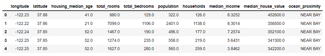
히스토그램으로 데이터 분석해보기

%matplotlib inline
import matplotlib.pyplot as plt
housing.hist(bins=50, figsize=(20,15))
save_fig("attribute_histogram_plots")
plt.show()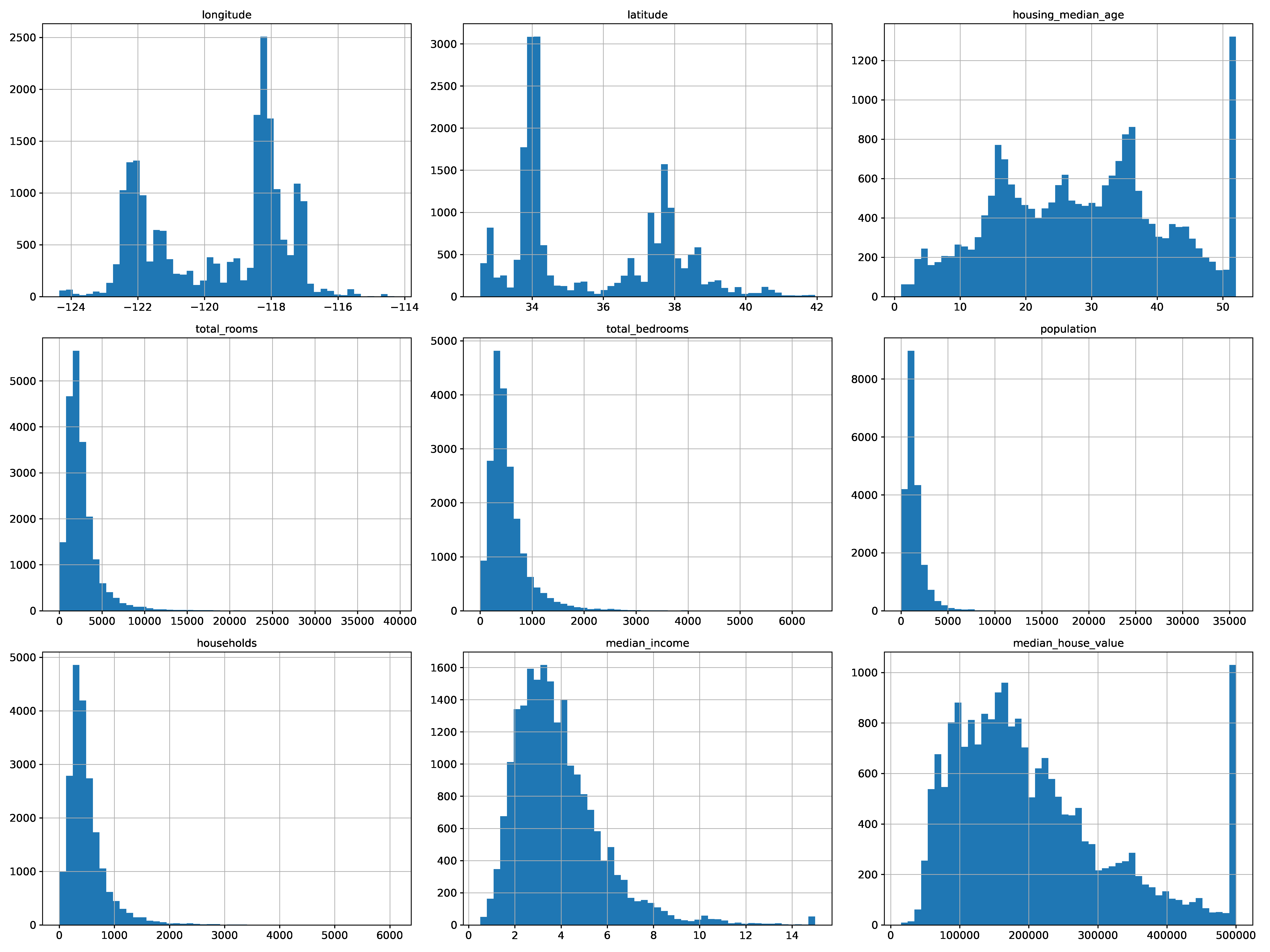

테스트 데이터셋 만들기

좋은 모델을 만들기 위해선 훈련에 사용되지 않고 모델평가만을 위해서 사용될 "테스트 데이터셋"을 따로 구분하는 것이 필요

계층적 샘플링(stratified sampling)
- 전체 데이터를 계층(strata)라는 동질의 그룹으로 나누고, 테스트 데이터가 전체 데이터를 잘 대표하도록 각 계층에서 올바른 수의 샘플을 추출

# 직관적으로, 집의 가격와 가계 수입이 관련이 있을 것으로 판단되므로
# median_income 변수를 사용해 전체 데이터를 계층화하자. 

# 연속형 변수를 5개 카테고리로 범주화
housing["income_cat"] = pd.cut(housing["median_income"],
                               bins=[0., 1.5, 3.0, 4.5, 6., np.inf],
                               labels=[1, 2, 3, 4, 5])
                               

from sklearn.model_selection import StratifiedShuffleSplit

split = StratifiedShuffleSplit(n_splits=1, test_size=0.2, random_state=42)
for train_index, test_index in split.split(housing, housing['income_cat']):
    strat_train_set = housing.loc[train_index]
    strat_test_set = housing.loc[test_index]

3. 데이터 이해를 위한 탐색과 시각화

지리적 데이터 시각화
- alpha 옵션을 사용해서 밀집된 영역은 더 진하게 표시해보자.
- s: 원의 반지름으로 인구 수를 표현
- c: 색상으로 가격을 표현

housing.plot(kind="scatter", x="longitude", y="latitude", alpha=0.4,
    s=housing["population"]/100, label="population", figsize=(10,7),
    c="median_house_value", cmap=plt.get_cmap("jet"), colorbar=True,
    sharex=False)
plt.legend()
save_fig("housing_prices_scatterplot")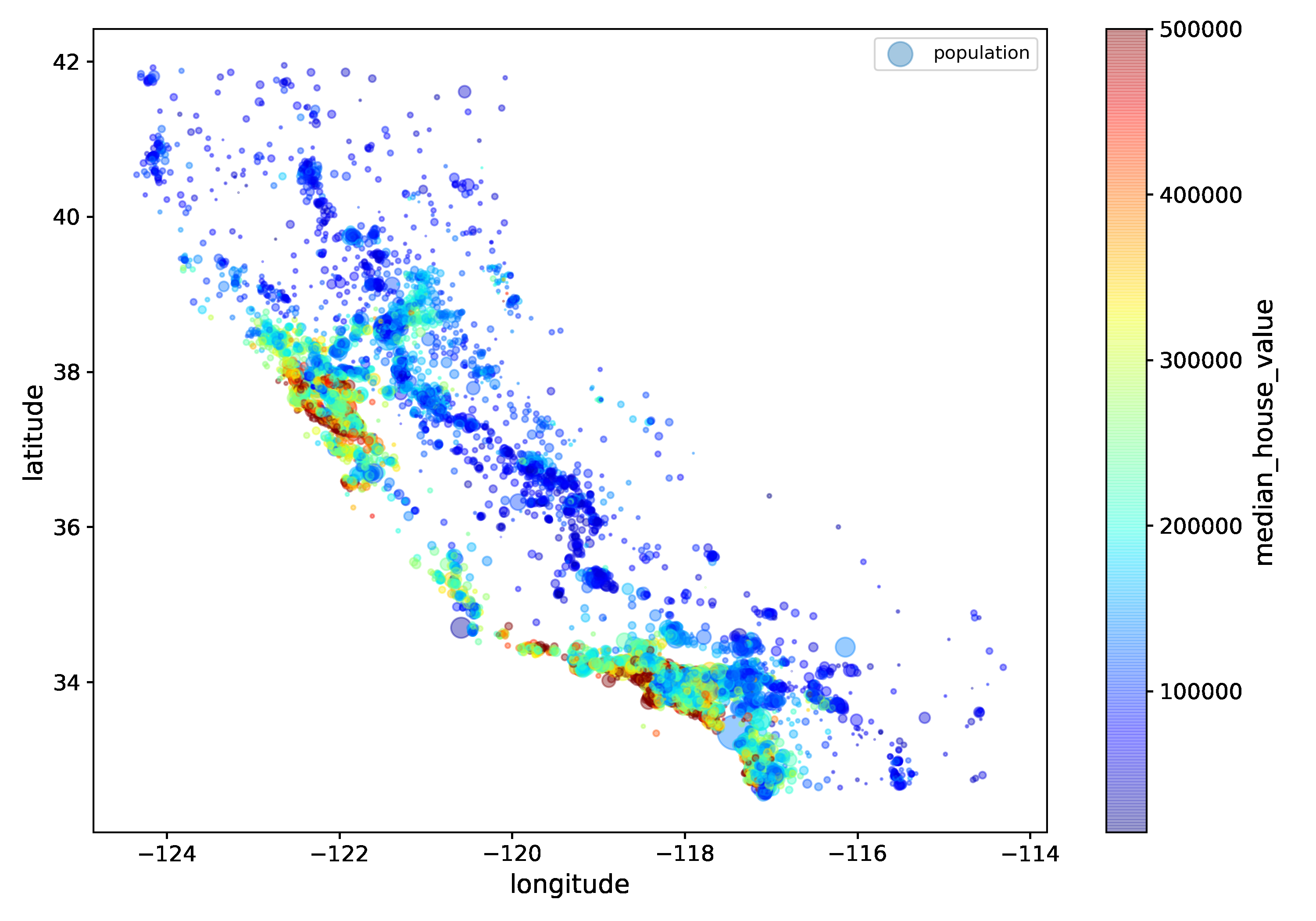

상관관계(Correlations) 관찰하기

corr_matrix = housing.corr()
corr_matrix["median_house_value"].sort_values(ascending=False)

## output
# median_house_value    1.000000
# median_income         0.687160
# total_rooms           0.135097
# housing_median_age    0.114110
# households            0.064506
# total_bedrooms        0.047689
# population           -0.026920
# longitude            -0.047432
# latitude             -0.142724
# Name: median_house_value, dtype: float64

scatter_matrix 사용

# from pandas.tools.plotting import scatter_matrix # For older versions of Pandas
from pandas.plotting import scatter_matrix

# 특성 몇 개만 살펴봄 
attributes = ["median_house_value", "median_income", "total_rooms",
              "housing_median_age"]
scatter_matrix(housing[attributes], figsize=(12, 8))
save_fig("scatter_matrix_plot")

특성 조합들 실험

여러 특성(feature, attribute)들의 조합으로 새로운 특성을 정의해볼 수 있다.

# 예를 들자면, 가구당 방 개수, 침대방(bedroom)의 비율, 가구당 인원

housing["rooms_per_household"] = housing["total_rooms"]/housing["households"]
housing["bedrooms_per_room"] = housing["total_bedrooms"]/housing["total_rooms"]
housing["population_per_household"]=housing["population"]/housing["households"]

corr_matrix = housing.corr()
corr_matrix["median_house_value"].sort_values(ascending=False)

## output
# median_house_value          1.000000
# median_income               0.687160
# rooms_per_household         0.146285
# total_rooms                 0.135097
# housing_median_age          0.114110
# households                  0.064506
# total_bedrooms              0.047689
# population_per_household   -0.021985
# population                 -0.026920
# longitude                  -0.047432
# latitude                   -0.142724
# bedrooms_per_room          -0.259984
# Name: median_house_value, dtype: float64

위에서 관찰할 수 있는 사실들?
- bedrooms_per_room: 집값과 강한 음의 상관관계 (집이 클수록 침실의 비율은 작아질 것)
- rooms_per_household: 집값과 양의 상관관계 (방이 많을수록 집이 클 것이고, 집이 크면 집값도 비쌀 것)

4. 머신러닝 알고리즘을 위한 데이터 준비

데이터 준비는 데이터 변환(data transformation)과정으로 볼 수 있다.

데이터 정제(Data Cleaning)

누락된 값(missing value, 결측치)을 다루는 방법들
- 해당 구역을 제거(행을 제거)
- 해당 특성을 제거(열을 제거)
- 어떤 값으로 채움(0, 평균, 중간값 등) 가장 추천하는 방법

# 결측치를 가지는 행들 샘플
sample_incomplete_rows = housing[housing.isnull().any(axis=1)].head() # True if there is a null feature

# option 1(행을 제거)
sample_incomplete_rows.dropna(subset=["total_bedrooms"])    

# option 2(열을 제거)
sample_incomplete_rows.drop("total_bedrooms", axis=1)   

# option 3(중앙값으로 채움)
median = housing["total_bedrooms"].median()
sample_incomplete_rows["total_bedrooms"].fillna(median, inplace=True)

SimpleImputer 사용하기

from sklearn.impute import SimpleImputer
imputer = SimpleImputer(strategy="median") # 중앙값으로 채우기

# 중간값은 수치형 특성에서만 계산될 수 있기 때문에 텍스트 특성을 제외한 복사본을 생성
housing_num = housing.drop("ocean_proximity", axis=1)

imputer.fit(housing_num)

# 학습된 imputer 객체를 사용해 누락된 값을 중간값으로 채울 수 있다.
X = imputer.transform(housing_num)

# X는 numpy array이므로 이를 다시 pandas DataFrame으로 바꾸자.
housing_tr = pd.DataFrame(X, columns=housing_num.columns,
                          index=housing.index)

Estimator, Transformer, Predictor 개념

추정기(estimator)
- 데이터셋을 기반으로 모델 파라미터들을 추정하는 객체(예를 들자면 imputer).
- 추정자체는 fit() method에 의해서 수행되고 하나의 데이터셋을 매개변수로 전달받는다.
- 지도학습의 경우 label을 담고 있는 데이터셋을 추가적인 매개변수로 전달한다.
변환기(transformer):
- (imputer같이) 데이터셋을 변환하는 추정기
- 변환은 transform() method가 수행하고 변환된 데이터셋을 반환한다.
예측기(predictor)
- 일부 추정기는 주어진 새로운 데이터셋에 대해 예측값을 생성할 수 있다.
- 예측기의 predict() method는 새로운 데이터셋을 받아 예측값을 반환한다.
- score() method는 예측값에 대한 평가지표를 반환한다.

텍스트와 범주형 특성 다루기

OrdinalEncoder
- "특성의 값이 비슷할수록 두 개의 샘플이 비슷하다"가 성립할 때 모델학습이 쉬워진다.

# 범주형 특성
housing_cat = housing[["ocean_proximity"]]

from sklearn.preprocessing import OrdinalEncoder

ordinal_encoder = OrdinalEncoder()
housing_cat_encoded = ordinal_encoder.fit_transform(housing_cat)

ordinal_encoder.categories_
## output
# [array(['<1H OCEAN', 'INLAND', 'ISLAND', 'NEAR BAY', 'NEAR OCEAN'], dtype=object)]

OneHotEncoder

from sklearn.preprocessing import OneHotEncoder

cat_encoder = OneHotEncoder(sparse=False)
housing_cat_1hot = cat_encoder.fit_transform(housing_cat)
housing_cat_1hot

나만의 변환기(Custom Transformers) 만들기

프로젝트를 위해 특별한 데이터 처리 작업을 해야 할 경우, 직접 변환기를 만들 수 있다. 반드시 구현해야 할 method는 fit()과 transform()이다.

아래의 custom tranformer는 rooms_per_household, population_per_household 두 개의 새로운 특성을 데이터셋에 추가하며 add_bedrooms_per_room = True로 주어지면 bedrooms_per_room 특성까지 추가한다. (add_bedrooms_per_room은 하이퍼파라미터로, 나중에 여러 조합을 테스트할 때 유용하다.)

from sklearn.base import BaseEstimator, TransformerMixin

# column index 저장
rooms_ix, bedrooms_ix, population_ix, households_ix = 3, 4, 5, 6

class CombinedAttributesAdder(BaseEstimator, TransformerMixin):
    def __init__(self, add_bedrooms_per_room = True): # no *args or **kargs
        self.add_bedrooms_per_room = add_bedrooms_per_room
    def fit(self, X, y=None):
        return self  # nothing else to do
    def transform(self, X): # X는 numpy array
        rooms_per_household = X[:, rooms_ix] / X[:, households_ix]
        population_per_household = X[:, population_ix] / X[:, households_ix]
        if self.add_bedrooms_per_room:
            bedrooms_per_room = X[:, bedrooms_ix] / X[:, rooms_ix]
            return np.c_[X, rooms_per_household, population_per_household,
                         bedrooms_per_room]
        else:
            return np.c_[X, rooms_per_household, population_per_household]

attr_adder = CombinedAttributesAdder(add_bedrooms_per_room=False)
housing_extra_attribs = attr_adder.transform(housing.values)


# numpy 데이터를 dataframe으로 변환
housing_extra_attribs = pd.DataFrame(
    housing_extra_attribs,
    columns=list(housing.columns)+["rooms_per_household", "population_per_household"],
    index=housing.index)
housing_extra_attribs.head()

특성 스케일링(Feature Scaling)

Min-max scaling
- 0과 1사이의 값이 되도록 조정
표준화(standardization)
- 평균이 0, 분산이 1이 되도록 만들어 줌(sklearn의 StandardScaler사용)

변환 파이프라인(Transformation Pipelines)

여러 개의 변환이 순차적으로 이루어져야 할 경우 Pipeline class를 사용하면 편리하다.

Pipeline 사용하기
- 이름, 추정기 쌍의 목록이 필요
- 마지막 단계를 제외하고 모두 변환기(즉, fit_transform() method를 가지고 있어야 함).
- 파이프라인의 fit() method를 호출하면 모든 변환기의 fit_transform() method를 순서대로 호출하면서 한 단계의 출력을 다음 단계의 입력으로 전달한다.
- 마지막 단계에서는 fit() method만 호출

from sklearn.pipeline import Pipeline
from sklearn.preprocessing import StandardScaler

num_pipeline = Pipeline([
        ('imputer', SimpleImputer(strategy="median")), # median으로 결측치 채우기
        ('attribs_adder', CombinedAttributesAdder()), # 새로운 특성 추가하기
        ('std_scaler', StandardScaler()), # 표준화하기
    ])

housing_num_tr = num_pipeline.fit_transform(housing_num)

ColumnTransformer로 각 열(column) 마다 다른 파이프라인을 적용
- 예를 들어 수치형 특성들과 범주형 특성들에 대해 별도의 변환이 필요한 경우

from sklearn.compose import ColumnTransformer

num_attribs = list(housing_num) # 수치형 특성들
cat_attribs = ["ocean_proximity"] # 범주형 특성

full_pipeline = ColumnTransformer([
        ("num", num_pipeline, num_attribs),
        ("cat", OneHotEncoder(), cat_attribs),
    ])

housing_prepared = full_pipeline.fit_transform(housing)

5. 모델 훈련

선형회귀모델(linear regression) 사용

from sklearn.linear_model import LinearRegression

lin_reg = LinearRegression()
lin_reg.fit(housing_prepared, housing_labels)

RMSE 측정

# 전체 훈련 데이터셋에 대한 RMSE를 측정
from sklearn.metrics import mean_squared_error

housing_predictions = lin_reg.predict(housing_prepared)
lin_mse = mean_squared_error(housing_labels, housing_predictions)
lin_rmse = np.sqrt(lin_mse)
lin_rmse

## output
# 68628.19819848923

훈련 데이터셋의 RMSE가 이 경우처럼 큰 경우, 과소적합(under-fitting)이라고 판단된다.

과소적합이 일어나는 이유?
- 특성들(features)이 충분한 정보를 제공하지 못함
- 모델이 충분히 강력하지 못함

DecisionTreeRegressor 사용

from sklearn.tree import DecisionTreeRegressor

tree_reg = DecisionTreeRegressor(random_state=42)
tree_reg.fit(housing_prepared, housing_labels)

housing_predictions = tree_reg.predict(housing_prepared)
tree_mse = mean_squared_error(housing_labels, housing_predictions)
tree_rmse = np.sqrt(tree_mse)
tree_rmse

## output
# 0.0

RandomForestRegressor 사용

from sklearn.ensemble import RandomForestRegressor

forest_reg = RandomForestRegressor(n_estimators=100, random_state=42)
forest_reg.fit(housing_prepared, housing_labels)

housing_predictions = forest_reg.predict(housing_prepared)
forest_mse = mean_squared_error(housing_labels, housing_predictions)
forest_rmse = np.sqrt(forest_mse)
forest_rmse

## output
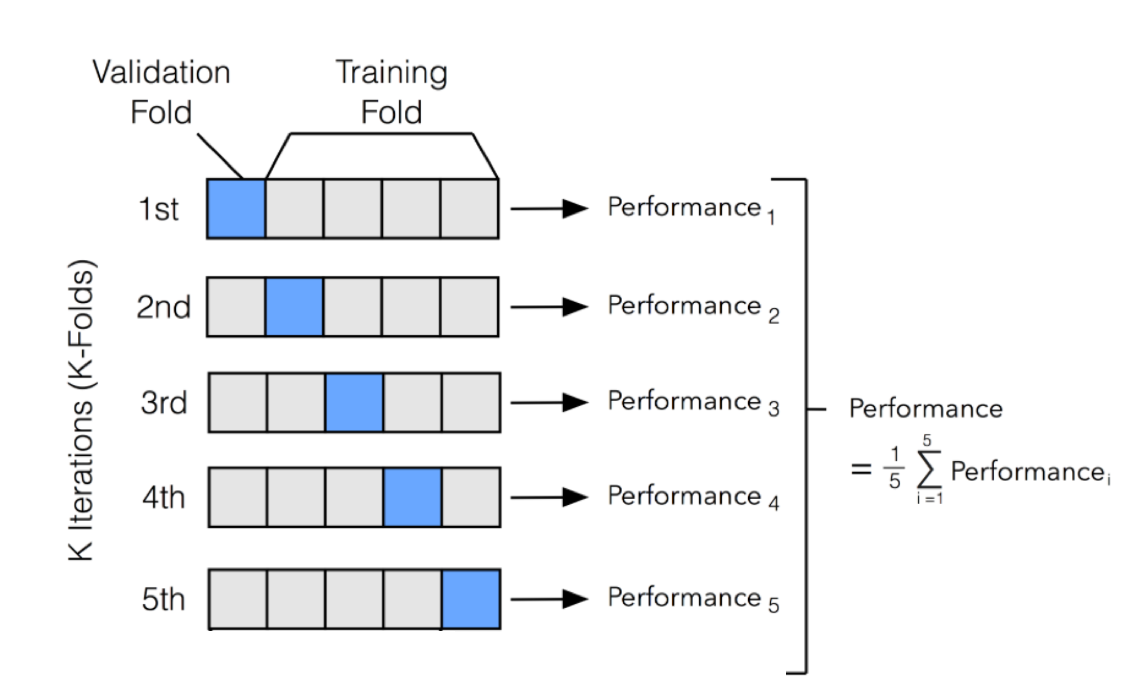
# 18603.515021376355

교차 검증(Cross-Validation)을 사용한 평가

from sklearn.model_selection import cross_val_score

def display_scores(scores):
    print("Scores:", scores)
    print("Mean:", scores.mean())
    print("Standard deviation:", scores.std())


# 결정트리모델에 대한 평가
scores = cross_val_score(tree_reg, housing_prepared, housing_labels,
                         scoring="neg_mean_squared_error", cv=10)
tree_rmse_scores = np.sqrt(-scores)
display_scores(tree_rmse_scores)

## output
# Scores: [70194.33680785 66855.16363941 72432.58244769 70758.73896782
#  71115.88230639 75585.14172901 70262.86139133 70273.6325285
#  75366.87952553 71231.65726027]
# Mean: 71407.68766037929
# Standard deviation: 2439.4345041191004


# 선형회귀모델에 대한 평가
lin_scores = cross_val_score(lin_reg, housing_prepared, housing_labels,
                             scoring="neg_mean_squared_error", cv=10)
lin_rmse_scores = np.sqrt(-lin_scores)
display_scores(lin_rmse_scores)

## output
# Scores: [66782.73843989 66960.118071   70347.95244419 74739.57052552
#  68031.13388938 71193.84183426 64969.63056405 68281.61137997
#  71552.91566558 67665.10082067]
# Mean: 69052.46136345083
# Standard deviation: 2731.6740017983498


# RandomForestRegressor에 대한 평가
forest_scores = cross_val_score(forest_reg, housing_prepared, housing_labels,
                                scoring="neg_mean_squared_error", cv=10)
forest_rmse_scores = np.sqrt(-forest_scores)
display_scores(forest_rmse_scores)

## output
# Scores: [49519.80364233 47461.9115823  50029.02762854 52325.28068953
#  49308.39426421 53446.37892622 48634.8036574  47585.73832311
#  53490.10699751 50021.5852922 ]
# Mean: 50182.303100336096
# Standard deviation: 2097.0810550985693

# RandomForestRegressor를 최종 모델로 채택한다.

6. 모델 세부 튜닝

모델의 종류를 선택한 후, 모델 학습을 위한 최적의 하이퍼파라미터를 찾는 과정

그리드 탐색(Grid Search); GridSearchCV 사용

from sklearn.model_selection import GridSearchCV

param_grid = [
    # try 12 (3×4) combinations of hyperparameters
    {'n_estimators': [3, 10, 30], 'max_features': [2, 4, 6, 8]},
    # then try 6 (2×3) combinations with bootstrap set as False
    {'bootstrap': [False], 'n_estimators': [3, 10], 'max_features': [2, 3, 4]},
  ]

forest_reg = RandomForestRegressor(random_state=42)
# train across 5 folds, that's a total of (12+6)*5=90 rounds of training 
grid_search = GridSearchCV(forest_reg, param_grid, cv=5,
                           scoring='neg_mean_squared_error',
                           return_train_score=True)
grid_search.fit(housing_prepared, housing_labels)

grid_search.best_estimator_

## output
# RandomForestRegressor(max_features=8, n_estimators=30, random_state=42)

랜덤 탐색(Randomized Search); RandomizedSearchCV 사용
- 하이퍼파라미터 조합의 수가 큰 경우에 유리하며, 지정한 횟수만큼만 평가한다.

from sklearn.model_selection import RandomizedSearchCV
from scipy.stats import randint

param_distribs = {
        'n_estimators': randint(low=1, high=200),
        'max_features': randint(low=1, high=8),
    }

forest_reg = RandomForestRegressor(random_state=42)
rnd_search = RandomizedSearchCV(forest_reg, param_distributions=param_distribs,
                                n_iter=10, cv=5, scoring='neg_mean_squared_error', random_state=42)
rnd_search.fit(housing_prepared, housing_labels)

rnd_search.best_estimator_

## output
# RandomForestRegressor(max_features=7, n_estimators=180, random_state=42)

특성 중요도, 에러 분석

feature_importances = grid_search.best_estimator_.feature_importances_

extra_attribs = ["rooms_per_hhold", "pop_per_hhold", "bedrooms_per_room"]
#cat_encoder = cat_pipeline.named_steps["cat_encoder"] # old solution
cat_encoder = full_pipeline.named_transformers_["cat"]
cat_one_hot_attribs = list(cat_encoder.categories_[0])
attributes = num_attribs + extra_attribs + cat_one_hot_attribs
sorted(zip(feature_importances, attributes), reverse=True)

## output
# [(0.36615898061813423, 'median_income'),
#  (0.16478099356159054, 'INLAND'),
#  (0.10879295677551575, 'pop_per_hhold'),
#  (0.07334423551601243, 'longitude'),
#  (0.06290907048262032, 'latitude'),
#  (0.056419179181954014, 'rooms_per_hhold'),
#  (0.053351077347675815, 'bedrooms_per_room'),
#  (0.04114379847872964, 'housing_median_age'),
#  (0.014874280890402769, 'population'),
#  (0.014672685420543239, 'total_rooms'),
#  (0.014257599323407808, 'households'),
#  (0.014106483453584104, 'total_bedrooms'),
#  (0.010311488326303788, '<1H OCEAN'),
#  (0.0028564746373201584, 'NEAR OCEAN'),
#  (0.0019604155994780706, 'NEAR BAY'),
#  (6.0280386727366e-05, 'ISLAND')]

7. 테스트 데이터셋으로 최종 평가하기

final_model = grid_search.best_estimator_

X_test = strat_test_set.drop("median_house_value", axis=1)
y_test = strat_test_set["median_house_value"].copy()

X_test_prepared = full_pipeline.transform(X_test)
final_predictions = final_model.predict(X_test_prepared)

final_mse = mean_squared_error(y_test, final_predictions)
final_rmse = np.sqrt(final_mse)

final_rmse

## output
# 47730.22690385927

8. 론칭, 모니터링, 시스템 유지 보수

상용환경에 배포하기 위해서 데이터 전처리와 모델의 예측이 포함된 파이프라인을 만들어 저장하는 것이 좋다.

full_pipeline_with_predictor = Pipeline([
        ("preparation", full_pipeline),
        ("linear", LinearRegression())
    ])

full_pipeline_with_predictor.fit(housing, housing_labels)
# full_pipeline_with_predictor.predict(some_data)

my_model = full_pipeline_with_predictor

import joblib
joblib.dump(my_model, "my_model.pkl")
#...
my_model_loaded = joblib.load("my_model.pkl")

론칭 후 시스템 모니터링
- 시간이 지나면 모델이 낙후되면서 성능이 저하
- 자동모니터링: 추천시스템의 경우, 추천된 상품의 판매량이 줄어드는지?
- 수동모니터링: 이미지 분류의 경우, 분류된 이미지들 중 일부를 전문가에게 검토시킴
- 결과가 나빠진 경우
- 데이터 입력의 품질이 나빠졌는지? 센서고장?
- 트렌드의 변화? 계절적 요인?

유지보수
- 정기적으로 새로운 데이터 수집(레이블)
- 새로운 데이터를 테스트 데이터로, 현재의 테스트 데이터는 학습데이터로 편입
- 다시 학습후, 새로운 테스트 데이터에 기반해 현재 모델과 새 모델을 평가, 비교

전체 프로세스에 고르게 시간을 배분해야 한다!

이다혜

하루하루 성장중

이전 포스트

[TIL Day24] Machine Learning 기초 - Decision Theory & Linear Regression

다음 포스트