--23.CNN Layer들.ipynb--
import numpy as np
import tensorflow as tf
Tensor 생성
Numpy 의 array 처럼 Tensor 객체를 다룰 수 있다.
tf.constant()
tf.constant([1, 2, 3])
tf.constant(((1, 2, 3), (4, 5, 6)))
tensor = tf.constant(np.array([10, 20, 30]))
tensor
Tensor의 정보들
tensor.shape
tensor.ndim
tensor.dtype
data type 정의
tf.constant([11, 22, 33], dtype=tf.uint8)
tf.constant([11, 22, 33], dtype=tf.float32)
data type 변환
tensor = tf.constant([11, 22, 33], dtype=tf.float32)
tensor
tf.cast(tensor, dtype=tf.uint8)
tensor # 원본은 변화 없다.
Tensor 안의 Numpy array 꺼내기
tensor.numpy() #방법1
np.array(tensor)
난수 생성
tf.random.normal([9])
tf.random.normal([3, 3])
tf.random.uniform([4, 4]) # [0,1) 사이의 균등분포 난수. 4 x 4 Tensor 0보다 크거나 같고 1보다 작은
데이터 준비
from tensorflow import keras
import matplotlib.pyplot as plt
import os
(train_x, trian_y), (test_x, test_y) = keras.datasets.fashion_mnist.load_data()
train_x.shape
test_x.shape
샘플 하나
image = train_x[0]
image.shape
plt.imshow(image, 'gray')
plt.show()
(28, 28) => (1, 28, 28, 1) (batch, height, width, channel)
image = image[tf.newaxis, ..., tf.newaxis]
image.shape
image.dtype
int 타입으로 모델에 집어넣으면 '에러' 난다!
image = tf.cast(image, dtype=tf.float32)
image.dtype
conv_layer = keras.layers.Conv2D(3, 3, 1, padding='same')
conv_layer
image를 레이어에 넣어주고 output을 확인해 볼 수 있다.
conv_output = conv_layer(image) # 입력 (1, 28, 28 , 1)
conv_output.shape
conv_layer = keras.layers.Conv2D(5, 3, 1, padding='same')
conv_output = conv_layer(image)
conv_output.shape
conv_layer = keras.layers.Conv2D(5, 3, 1, padding='VALID')
conv_output = conv_layer(image)
conv_output.shape # (1, 26, 26, 5)
첫번째 채널 하나만 시각화 해보자
plt.imshow(conv_output[0, :, :, 0], 'gray')
plt.show()
※ 결과들이 달라보이는 이유, 애시당초 filter의 weight들은 random 하게 초기화 되어 동작하기 때문.
원본 이미지와 비교
plt.subplot(1, 2, 1)
plt.imshow(image[0, :, :, 0], 'gray')
plt.subplot(1, 2, 2)
plt.imshow(conv_output[0, :, :, 0], 'gray')
plt.show()
원본 이미지 값의 범위
np.min(image), np.max(image)
Conv2D 를 거치면서 변한 값들
np.min(conv_output), np.max(conv_output)
layer의 get_weights()
weights = conv_layer.get_weights() # array 2개가 담긴 list 리턴
print(weights[0].shape, weights[1].shape) # (3, 3, 1, 5) (5,)
[0] 번째 weight
[1] 번째 bias
weights
layer의 param 개수
weights[0].size + weights[1].size
시각화
1. 이미지 히스토그램 2. filter 3. output
plt.figure(figsize=(15, 5))
1. 히스토그램
plt.subplot(131)
plt.hist(conv_output.numpy().ravel())
2. filter
plt.subplot(132)
plt.title(weights[0].shape)
plt.imshow(weights[0][:, :, 0, 0], 'gray') # 맨 앞 filter 의 (3, 3) 값만 시각화
3. output
plt.subplot(133)
plt.title(conv_output.shape)
plt.imshow(conv_output[0, :, :, 0], 'gray')
plt.colorbar()
plt.show()
ReLU 레이어 만들기
act_layer = tf.keras.layers.ReLU()
act_output = act_layer(conv_output)
print(act_output.shape)
act_output
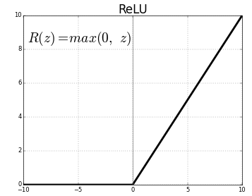
0 미만의 값들은 0으로 바뀌었다!
np.min(act_output), np.max(act_output)
시각화
1. 이미지 히스토그램 3. output
plt.figure(figsize=(15, 5))
1. 히스토그램
plt.subplot(121)
plt.hist(act_output.numpy().ravel())
3. output
plt.subplot(122)
plt.title(act_output.shape)
plt.imshow(act_output[0, :, :, 0], 'gray')
plt.colorbar()
plt.show()
act_output.shape
pool_layer = tf.keras.layers.MaxPool2D(2) # 2 = pool_size=(2,2)
pool_output = pool_layer(act_output)
print(pool_output.shape)
시각화
1. 이미지 히스토그램 3. output
plt.figure(figsize=(15, 5))
1. 히스토그램
plt.subplot(121)
plt.hist(pool_output.numpy().ravel())
3. output
plt.subplot(122)
plt.title(pool_output.shape)
plt.imshow(pool_output[0, :, :, 0], 'gray')
plt.colorbar()
plt.show()
pool_output.shape
flat_layer = tf.keras.layers.Flatten()
flat_output = flat_layer(pool_output)
print(flat_output.shape)
"""
(1, 845) <= 왜 2차원? 앞의 1은 batch 차원
"""
None
시각화
1. 이미지 히스토그램 3. output
plt.figure(figsize=(10, 5))
1. 히스토그램
plt.subplot(211)
plt.hist(flat_output.numpy().ravel())
3. output
plt.subplot(212)
plt.title(flat_output.shape)
plt.imshow(flat_output[:, :])
plt.show()