SIFT - 5 Minutes with Cyrill

참조영상

SIFT(Scale Invariant Feature Transform)
: 이미지의 크기나 회전에 불변하는 특징을 추출하는 알고리즘
: 서로 다른 두 이미지에서 SIFT 특징을 각각 추출한 다음에 서로 가장 비슷한 특징끼리 매칭해주면 두 이미지에서 대응되는 부분을 찾을 수 있다는 것이 기본 원리

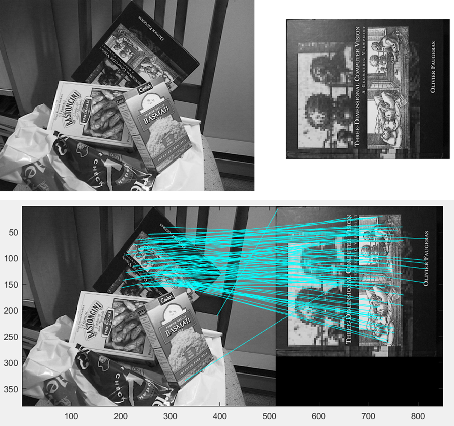다음 그림과 같이 크기와 회전은 다르지만,
일치하는 내용을 갖고 이미지에서 동일한 물체를 찾아 매칭해줄 수 있는 알고리즘

이미지의 크기도 다르고, 책이 회전된 정도도 다르고, 물체들에 가려져 있는데도 불구하고 일치되는 부분을 잘 매칭해준 것을 확인 (occlusion)😄
⇒ SIFT의 장점
++NCC는 occlusion인 경우는 다루지 못했다.

---

Motivation

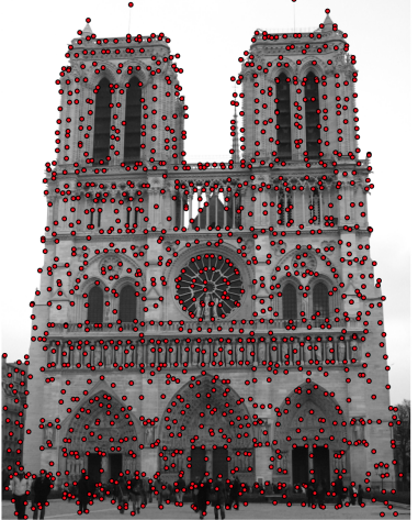locally distinct한 point들을 표시한 사진
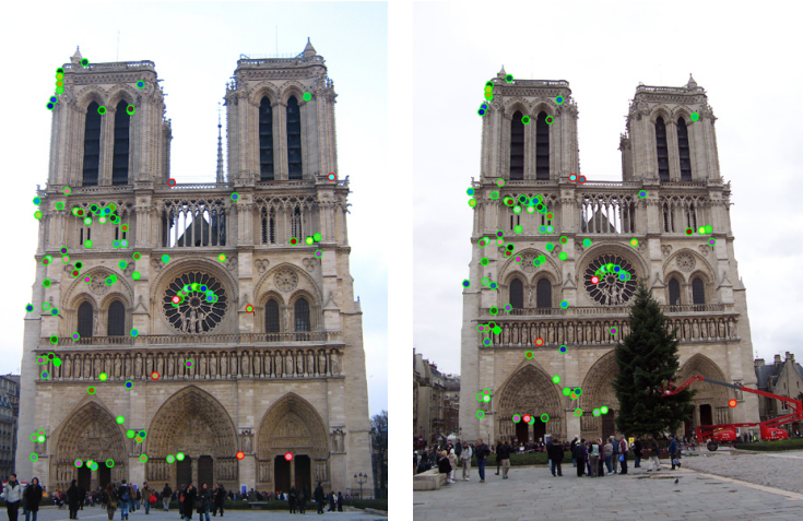keypoint들을 표시한 사진(이미지의 크기나 회전에 불변하는 특징)

---

Visual Features: KeyPoints and Descriptors

Keypoint
: (locally) distinct location in an image
: noise, 회전, 크기변환, 밝기변환에 강인한 point
: 이 조건에 맞는 특징점 중 하나를 코너점이라고 얘기할 수 있음

코너점이란?

상하좌우로 움직였을 때, 모두 큰 변화가 일어나는 곳

Descriptors
: keypoint를 설명하는 방식 - 128개의 숫자
: keypoint 주변의 local structure 요약
하나의 keypoint는 다음과 같은 하나의 vector = descriptor로 표현될 수 있음

---

Today’s Topics

---

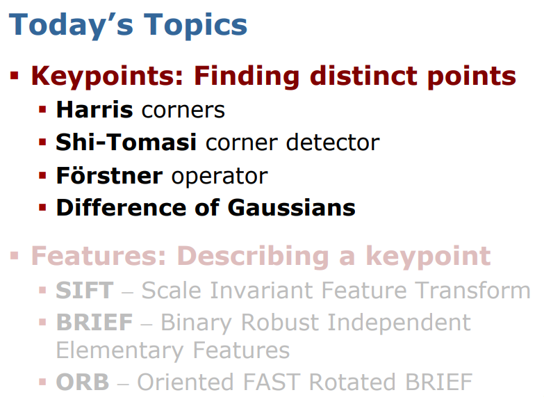
Keypoints : Part 1 _ Corners

Corners & Edges

• corners는 translation, rotation, illumination에 불변함
• corner
  : roughly orthogonal directions(직교방향)의 2개의 edges
• edges
  : sudden brightness change
  ex. bright→dark, dark→bright

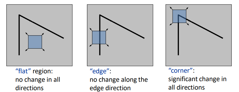
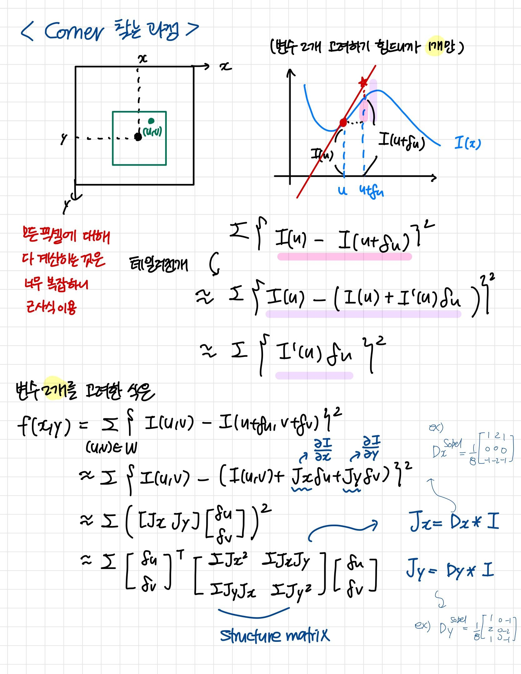
Finding Corners

• corners 찾기 위해서, 우리는 two directions에서 intensity changes를 찾아야 함
• $(x,y)$ 주변의 neighbor pixel의 SSD를 계산하기
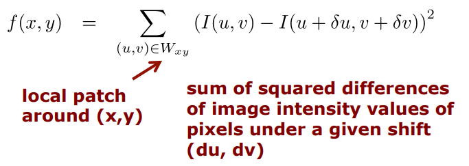  새롭게 옮겨진 위치에서의 값과 원래 위치에서의 값의 차를 구한 후 제곱한 식이다. (값이 클수록 변화가 크다는 것)

Talyor expansion

하지만,, 모든 픽셀을 계산하는 것은 좋지 못한 방법 ㅠ.ㅠ 따라서 제안된 것이 Talyor expansion

Talyor expansion
: 어떤 함수 f(x)를 다항함수로 근사시키는 것

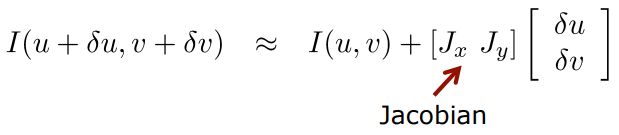Taylor approximation은 다음과 같은데..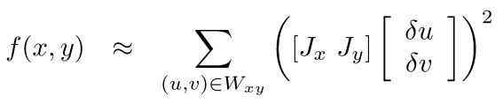matrix form으로 쓰면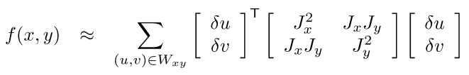sum의 기호를 matrix 안으로 쓰면

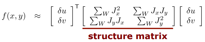
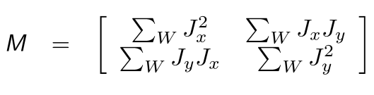
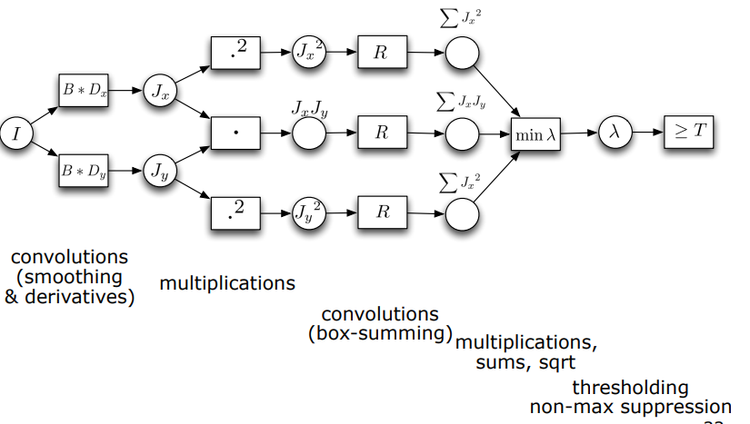
Structure Matrix

Structure Matrix
: first derivative에 대한 모든 정보를 담고 있는 가장 중요한 식이겠지!

• edges와 corners를 찾아내는 key와 같은 역할
• image gradients로부터 만들어짐
  

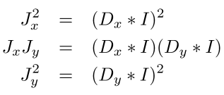
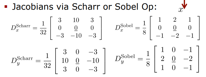
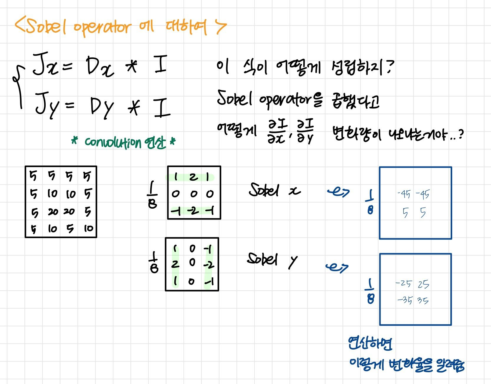
Computing the Structure Matrix

• Jacobians는 Scharr 또는 Sobel과 같은 gradient kernel를 이용하여 convolution으로 계산됨
  

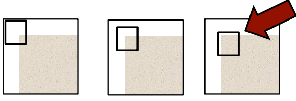
Structure Matrix Examples

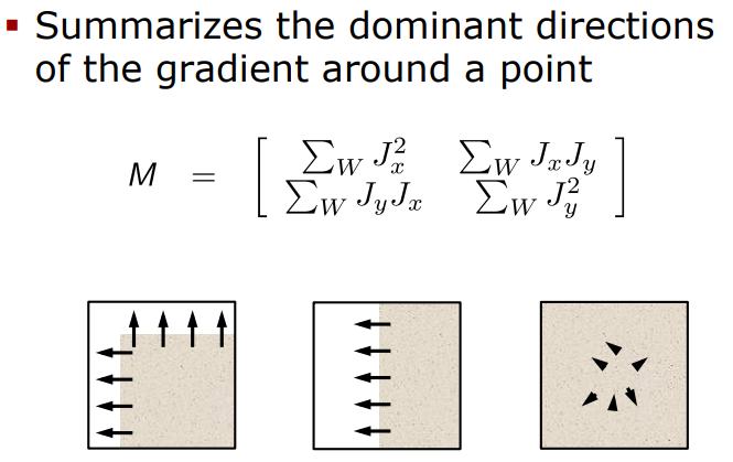
• 첫번째 사진: gradient가 X방향과 Y방향 모두 있기 때문에 가장 good
• 두번째 사진: gradient가 한 방향밖에 없기 때문에 별로 좋지 않음
  (가로 방향으로는 localize할 수 있지만, 세로 방향으로는 할 수 없으므로)
• 세번째 사진: intensity value 차이가 없기 때문에 제일 bad - local structure을 많이 갖지 않음
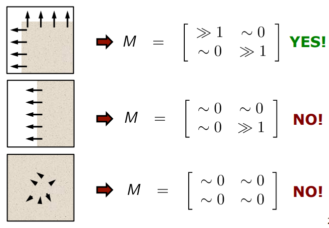  locally distinct라는 것의 정의는 첫번째만 !

  KEY IDEA
  structure matrix가 2개의 large eigenvalue(고유값)을 가질 때에만 !
  points를 corners라고 생각하라.

---

Harris, Shi-Tomasi & Forstner

corner을 정의하기 위한 3개의 비슷한 연구들이 있었음

• 1987: Forstner
• 1988: Harris
• 1994: Shi-Tomasi

모든 연구는 structure matrix를 기반으로 point가 corner인지 아닌지 결정할 때 서로 다른 기준(criterion) 사용
Fostner은 subpixel estimation 방법을 사용

---

1. Harris Corner Criterion

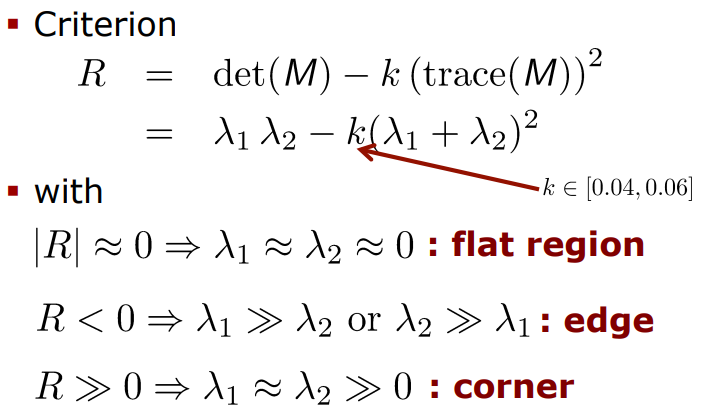$\lambda_1, \lambda_2$ : 고윳값(eigenvalue)를 의미함

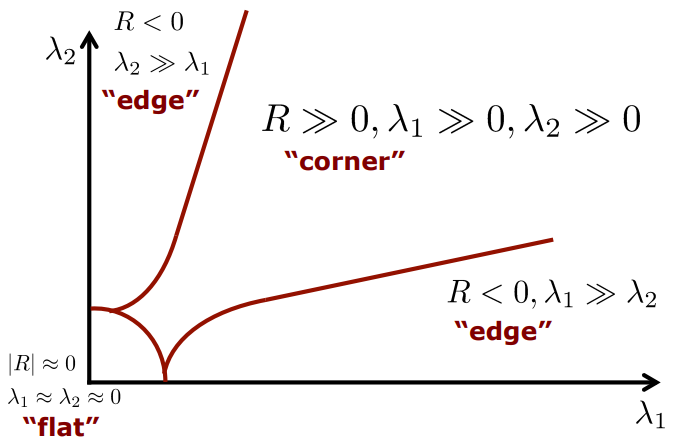
2. Shi-Tomasi Corner Detector

대부분의 libraries는 Shi-Tomasi를 default corner detector로 사용한다. (e.g. openCV)
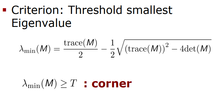기준점이 될 가장 작은 eigenvalue값을 구함

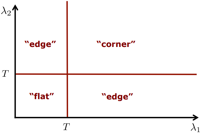
3. Forstner Operator Criterion

Harris corner dector 방법과 매우 비슷
sub-pixel estimation의 확장

Non-Maxima Supression

local region 안에서, maximum value($R$ or $\lambda_{min}$)로 position을 찾고 이 point를 선택함
3개의 그림 중에 무엇이 가장 best일까?
3번째 사진!
number of gradients가 더 크기 때문에

---

Summary Corner Detection

여기서는 Shi-Tomasi를 사용하였음

---

Keypoints : Part 2 _ Difference of Gaussians(DoG)

corner detection의 variant(또 다른 형태)
corners, edges, blobs에 대한 반응을 제공

blob
: 주로 constant region이지만, surroundings와 차이가 있는 곳

Keypoints

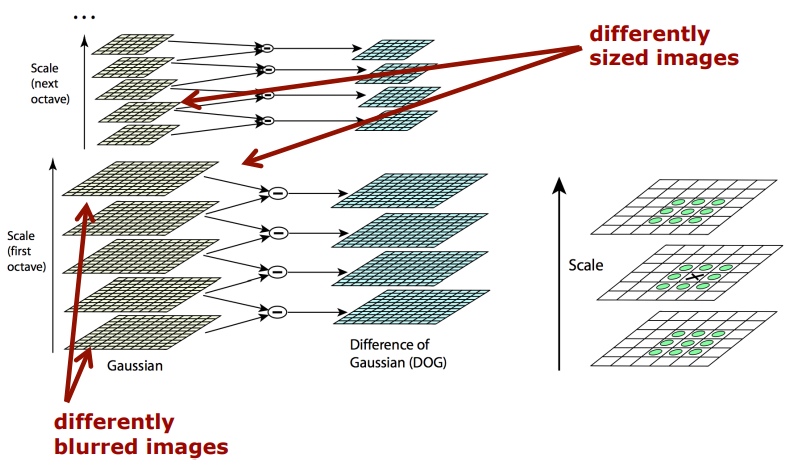
: Difference of Gaussians(DoG) over Scale-Space Pyramid

Procedure

다양한 이미지들은 pyramid levels 거쳐서...
(STEP1) Gaussian smoothing : blur 처리 하는 것
(STEP2) Difference-of-Gaussians(DoG)
(STEP3) maxima suppression at edges

Illustration

Difference of Gaussians (DoG)

• 다르게 blurred된 images를 서로 뺀 결과는 다음과 같이 나와

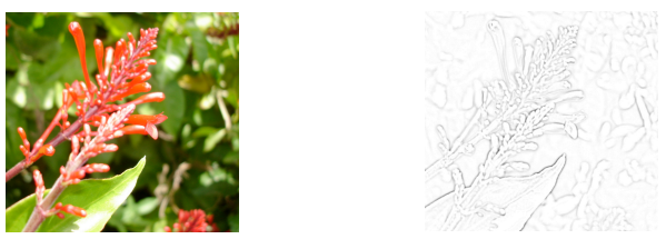
  왼쪽 사진이 원본이고
  오른쪽 사진이 blurred된 정도가 다른 두 image를 뺀 결과

• corners, edges, other detail에 대한 가시성이 더 높아진 것을 확인해볼 수 있음 😄
• DoG는 band-pass filter와 같은 역할을 함
  • band-pass filter
    : 특정한 주파수만 통과시키는 filter

Scale Space Representation

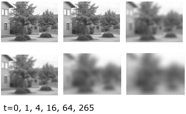Keypoints는 different (smoothing) scales을 걸쳐 DoG의 결과로 얻게 되는 극값(extrema)

---

Summary

• locally distinct points를 찾을 때 2가지 접근법이 존재
  1. Corners via structure matrix
     1. Harris
     2. Shi-Tomasi
     3. Forstner
  2. Difference of Gaussians(DoG)
     1. scale과 blur에 걸쳐서 계속 반복
     2. corner과 blob를 찾기

---

한눈에 정리

참고자료

• SIFT (Scale Invariant Feature Transform)의 원리
• SIFT 알고리즘