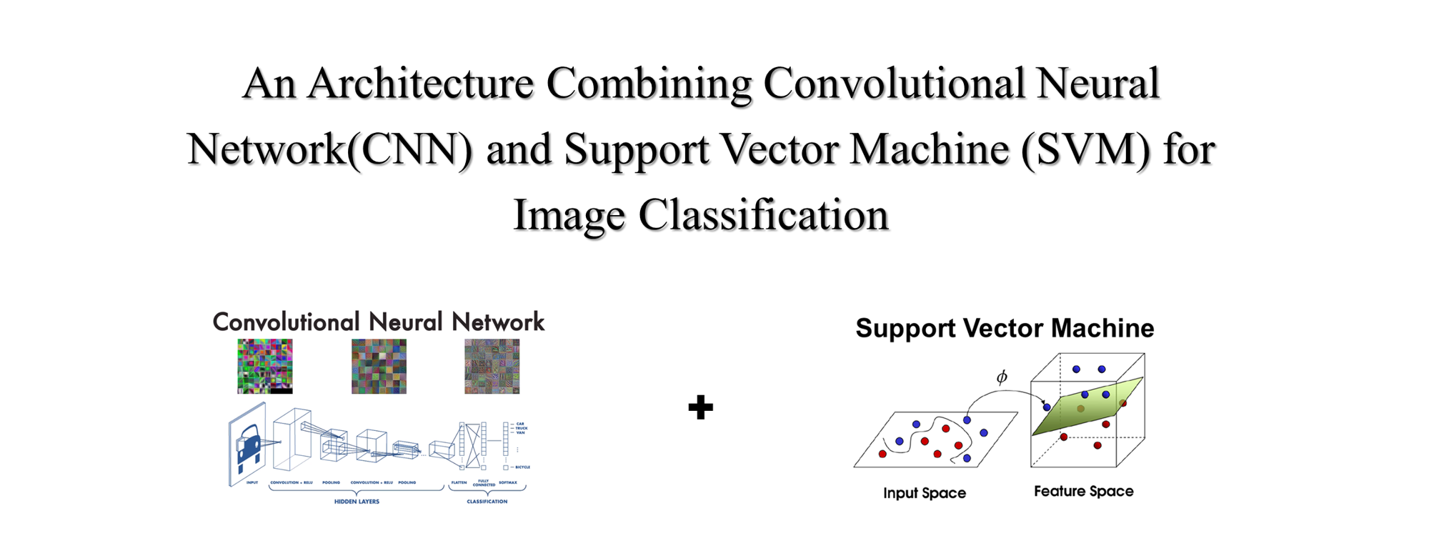
[Paper Review] An Architecture Combining Convolutional Neural Network(CNN) and Support Vector Machine(SVM) for Image Classification
오늘 리뷰/번역/구현할 논문은 "Abien Fred M. Agarap" 저자가 쓴 논문으로, "Yichuan Tang"의 "Deep Learning using Linear Support Vector Machines"을 보고 inspired되어 연구하게 되었다고 한다. 하단의 참고 논문 소스에 해당 논문 링크와 이번 논문의 링크를 첨부였다.
(참고) 논문 소스
- Deep Learning using Linear Support Vector Machines (클릭)
- An Architecture Combining Convolutional Neural Network (CNN) and Support Vector Machine (SVM) for Image Classification (클릭)
Abstract
-
CNN(합성곱신경망)은 Hidden layer들과 learnable parameter들로 구성되어 있으며, 각 뉴런에서는 input을 받으면 이를 내적하고, 비선형성을 더해준다. Raw Image와 해당 class score를 이어주는 매개체의 역할을 수행한다. (주로 CNN 마지막 단에는 softmax함수가 이용이 된다.
-
하지만, 몇몇 논문들은 위와 같은 방법론에 문제를 제기하였다:
- Abien Fred Agarap. 2017. A Neural Network Architecture Combining Gated Recurrent Unit (GRU) and Support Vector Machine (SVM) for Intrusion Detection in Network Traffic Data. arXiv preprint arXiv:1709.03082 (2017).
- Abdulrahman Alalshekmubarak and Leslie S Smith. 2013. A novel approach combining recurrent neural network and support vector machines for time series classification. In Innovations in Information Technology (IIT), 2013 9th International Conference on. IEEE, 42–47
- Yichuan Tang. 2013. Deep learning using linear support vector machines. arXiv preprint arXiv:1306.0239 (2013).
-
위에서 보여준 논문들은 공통적으로 linear SVM을 이용하는 것을 제안한다. 이에 저자는 CNN단에 Softmax 대신 SVM을 이용하여 분석을 수행한다.
-
MNIST
- CNN-SVM : 99.04%
- CNN-Softmax : 99.23%
-
MNIST-Fasion
- CNN-SVM : 90.72%
- CNN-Softmax : 91.86%
-
저자는 성능은 비록 조금 낮을 수 있을지라도, 좀 더 고도화된 CNN을 이용하면 성능을 더욱 더 향상시킬 수 있을 것이라고 주장한다.
💡 리뷰 논문 선정 이유
해당 논문에서는 이를 이용하여 State-of-the-art(SOTA)를 찍지는 않지만, 후에 다양한 Vision 분야에서 마지막 단에 SVM Classifier를 사용하기에 근간이 된 논문을 선정하게 되었다. 최근 연구에 있어서 모델에 간단한 변화를 (더해)줌으로써 모델의 성능을 향상시킬 수 있을까 하는 고민에 찾아보고 정리해보게 되었다.
1. Introduction
- 위에 Abstract에서 간단히 소개했듯이 NeuralNet(인공신경망)에 softmax이외에 다른 방법론(Ex. SVM)을 적용하는 연구들이 진행되어 왔다.
- Abien Fred Agarap. 2017. A Neural Network Architecture Combining Gated Recurrent Unit (GRU) and Support Vector Machine (SVM) for Intrusion Detection in Network Traffic Data. arXiv preprint arXiv:1709.03082 (2017).
- Abdulrahman Alalshekmubarak and Leslie S Smith. 2013. A novel approach combining recurrent neural network and support vector machines for time series classification. In Innovations in Information Technology (IIT), 2013 9th International Conference on. IEEE, 42–47
- Yichuan Tang. 2013. Deep learning using linear support vector machines. arXiv preprint arXiv:1306.0239 (2013).
- 이러한 연구들에서 ANN에 softmax를 적용하는 것보다, SVM을 적용하는 것이 더 좋다는 결과들이 나왔다. (이진 판별(binary classification) 한정, multinomial case의 경우 one-versus-all 방식 채용)
- 해당 논문에서는 2013년에 나온 "Deep learning using linear support vector machines" 논문에서 CNN모델을 좀 더 쉽고 간편한 2-Conv Layer with Max Pooling모델을 사용한다.
2. Metodology
2.1 Machine Intelligence Library
- 해당 논문은 Google의 Tensorflow을 이용하여 연구를 진행하였다.
- 이번 논문 구현에 있어서는 최근 가장 많이 사용되는 PyTorch를 이용하여 논문구현을 수행해보았다.
# Load Libraries
import torch
import torch.nn as nn
import torchvision.datasets as datasets
import torchvision.transforms as transforms
import torch.nn.init
from torch.utils.data import Dataset
from torch.autograd import Variable
from PIL import Image
from torch.utils.data import DataLoader
import matplotlib.pyplot as plt
import helper

# GPU 설정
device = 'cuda' if torch.cuda.is_available() else 'cpu'

# 랜덤 시드 고정
torch.manual_seed(123)

# GPU 사용 가능일 경우 랜덤 시드 고정
if device == 'cuda':
    torch.cuda.manual_seed_all(123)

# Define a transform to normalize the data
transform = transforms.Compose([transforms.ToTensor(), transforms.Normalize(mean=(0.5,), std=(0.5,))])
2.2 The Dataset
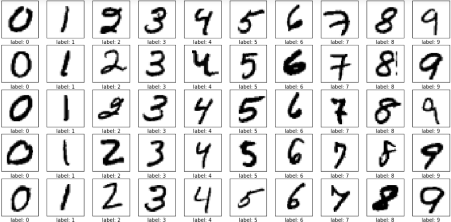
- MNIST : 10-class classification problem having 60,000 training examples, and 10,000 test cases – all in grayscale
- Fashion-MNIST : the same number of classes, and the same color profile as MNIST
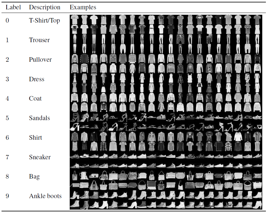
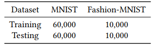
Table 1: Dataset distribution for both MNIST and Fashion-MNIST
Import fashion-MINIST
# Download and load the training data
fashion_trainset = datasets.FashionMNIST('~/.pytorch/F_MNIST_data/', download=True, train=True, transform=transform)
fashion_trainloader = torch.utils.data.DataLoader(fashion_trainset, batch_size=128, shuffle=True)

# Download and load the test data
fashion_testset = datasets.FashionMNIST('~/.pytorch/F_MNIST_data/', download=True, train=False, transform=transform)
fashion_testloader = torch.utils.data.DataLoader(fashion_testset, batch_size=128, shuffle=True)
Import MINIST
# Download and load the training data
mnist_trainset = datasets.MNIST('~/.pytorch/MNIST_data/', download=True, train=True, transform=transform)
mnist_trainloader = torch.utils.data.DataLoader(mnist_trainset, batch_size=128, shuffle=True)

# Download and load the test data
mnist_testset = datasets.MNIST('~/.pytorch/MNIST_data/', download=True, train=False, transform=transform)
mnist_testloader = torch.utils.data.DataLoader(mnist_testset, batch_size=128, shuffle=True)- 별도의 전처리는 수행하지 않는다. (No normalization or dimensionality reduction)
2.3 Support Vector Machine(SVM)
- Support Vector Machine(SVM)은 C. Cortes and V. Vapnik에 의해 개발된 이진분류 방법론으로, 최적의 초평면(f (w, x) = w · x + b)을 찾는 데에 의의를 둔다. 초평면은 서로 다른 두 class를 분류해준다.
- SVM은 해당 식을 최적화하여 W parameter를 학습한다.
- L1-SVM
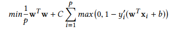
- 는 Manhattan norm(L1 norm), C는 penalty parameter, y'는 실제 y값, +b는 예측 y값이다.
- L2-SVM
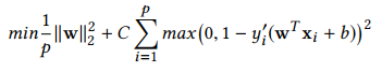
- 는 Euclidean norm(L2 norm), C는 penalty parameter, y'는 실제 y값, +b는 예측 y값이다.
- L1-SVM
class SVM:
		# set learning_rate, lambda, n iterations
    def __init__(self, learning_rate=0.001, lambda_param=0.01, n_iters=1000):
        self.lr = learning_rate
        self.lambda_param = lambda_param
        self.n_iters = n_iters
        self.w = None
        self.b = None

		# SVM fit function
    def fit(self, X, y):
        n_samples, n_features = X.shape

        y_ = np.where(y <= 0, -1, 1)

        self.w = np.zeros(n_features)
        self.b = 0

        for _ in range(self.n_iters):
            for idx, x_i in enumerate(X):
                condition = y_[idx] * (np.dot(x_i, self.w) - self.b) >= 1
                if condition:
                    self.w -= self.lr * (2 * self.lambda_param * self.w)
                else:
                    self.w -= self.lr * (2 * self.lambda_param * self.w - np.dot(x_i, y_[idx]))
                    self.b -= self.lr * y_[idx]

		# SVM predict function
    def predict(self, X):
        approx = np.dot(X, self.w) - self.b
        return np.sign(approx)
2.4 Convolutional Neural Network(CNN)
- Convolutional Neural Network(CNN)은 컴퓨터 비전에서 많이 쓰이는 deep feed-forward artificial neural network로, MLP 뿐만 아니라 convolutional layers, pooling, 그리고 비선형 activation function인 tanh, sigmoid, ReLU 등이 쓰인다.
- 본 연구에서는 다음과 같은 기본 CNN모델을 이용한다.
- 5x5x1 size filter
- 2x2 max pooling
- RELU as activation function (threshold = 0)
- 10번째 layer단에서 convolutional softmax 대신 L2-SVM을 이용한다. ( y ∈ {-1, +1}, adam optimizer 이용)
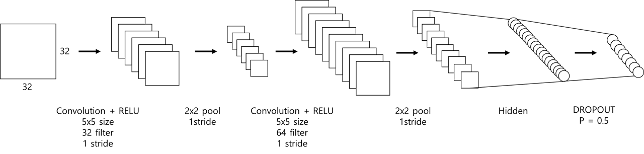
저자가 이용한 모델 구조(직접 제작)
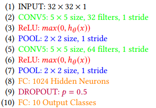
저자가 이용한 모델 구조(논문 수록)
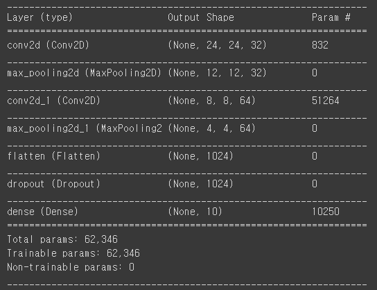
저자가 이용한 모델 구조(직접 구현)
CNN model
class CNN(torch.nn.Module):

    def __init__(self):
        super(CNN, self).__init__()
        self.drop_prob = 0.5

        # define layer1
        self.layer1 = torch.nn.Sequential(
            torch.nn.Conv2d(1, 32, kernel_size=5, stride=1),
            torch.nn.ReLU(),
            torch.nn.MaxPool2d(kernel_size=2, stride=1))

        # define layer2
        self.layer2 = torch.nn.Sequential(
            torch.nn.Conv2d(32, 64, kernel_size=5, stride=1),
            torch.nn.ReLU(),
            torch.nn.MaxPool2d(kernel_size=2, stride=1))

        # define fully connected layer (1024)
        self.fc1 = torch.nn.Linear(18 * 18 * 64, 1024, bias=True)
        torch.nn.init.xavier_uniform_(self.fc1.weight)
        self.layer3 = torch.nn.Sequential(
            self.fc1,
            torch.nn.Dropout(p= self.drop_prob))


        # define fully connected layer (10 classes)
        self.fc2 = torch.nn.Linear(1024, 10, bias=True)
        torch.nn.init.xavier_uniform_(self.fc2.weight)

    # define feed-forward
    def forward(self, x):
        out = self.layer1(x)
        out = self.layer2(out)
        out = out.view(out.size(0), -1)   # Flatten them for FC
        out = self.layer3(out)
        out = self.fc2(out)
        return out
CNN + SVM model (multi-Class Hinge Loss)
class multiClassHingeLoss(nn.Module):
def __init__(self, p=1, margin=1, weight=None, size_average=True):
super(multiClassHingeLoss, self).__init__()
self.p=p
self.margin=margin
self.weight=weight
self.size_average=size_average
# define feed-forward
def forward(self, output, y):`
output_y=output[torch.arange(0,y.size()[0]).long().cuda(),y.data.cuda()].view(-1,1)
# output - output(y) + output(i)
loss=output-output_y+self.margin
# remove i=y items
loss[torch.arange(0,y.size()[0]).long().cuda(),y.data.cuda()]=0
# apply max function
loss[loss<0]=0
# apply power p function
if(self.p!=1):
loss=torch.pow(loss,self.p)
# add weight
if(self.weight is not None):
loss=loss*self.weight
# sum up
loss=torch.sum(loss)
if(self.size_average):
loss/=output.size()[0]
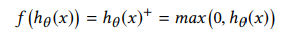
return loss💡 잠깐!! hinge loss란?
- 학습데이터 각각의 범주를 구분하면서 데이터와의 거리가 가장 먼 결정경계(decision boundary)를 찾기 위해 고안된 손실함수의 한 부류. 이로써 데이터와 경계 사이의 마진(margin)이 최대화된다.
- 이진 분류문제에서 모델의 예측값 y′(스칼라), 학습데이터의 실제값 y (-1 또는 1) 사이의 hinge loss는 아래와 같이 정의된다.
2.5 Data Analysis
- 2개의 phase(train/test)
- 2개의 dataset(MNIST, fashion-MNIST)
3. Experiments
- 아래 그림은 각각의 데이터셋에 대하여 설정해준 Hyper parameter 정보들이다.
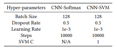
Table 2: Hyper-parameters used for CNN-Softmax and CNNSVM models.
Set hyper-parameter
learning_rate = 0.001
training_epochs = 50
# training_epochs = 10000
# 해당 논문에서는 만번의 epoch를 수행했지만 computation power로 인해 epoch 50회 수행
batch_size = 128
Make Model for MNIST Data (CNN)
# MNIST CNN 모델 정의
mnist_model = CNN().to(device)

criterion = torch.nn.CrossEntropyLoss().to(device)
optimizer = torch.optim.Adam(mnist_model.parameters(), lr=learning_rate)

total_batch = len(mnist_trainloader)
print('총 배치의 수 : {}'.format(total_batch))
Make Model for MNIST Data (CNN + SVM)
# MNIST CNN+SVM 모델 정의
minst_SVM_model = CNN().to(device)

criterion = multiClassHingeLoss().to(device)
optimizer = torch.optim.Adam(minst_SVM_model.parameters(), lr=learning_rate)

total_batch = len(mnist_trainloader)
print('총 배치의 수 : {}'.format(total_batch))
Make Model for fashion-MNIST Data (CNN)
# fashion-MNIST CNN 모델 정의
fashion_model = CNN().to(device)

criterion = torch.nn.CrossEntropyLoss().to(device)    # 비용 함수에 소프트맥스 함수 포함되어져 있음.
optimizer = torch.optim.Adam(fashion_model.parameters(), lr=learning_rate)

total_batch = len(fashion_trainloader)
print('총 배치의 수 : {}'.format(total_batch))
Make Model for fashion-MNIST Data (CNN + SVM)
# fashion-MNIST CNN + SVM 모델 정의
fashion_SVM_model = CNN().to(device)

criterion = multiClassHingeLoss().to(device)
optimizer = torch.optim.Adam(fashion_SVM_model.parameters(), lr=learning_rate)

total_batch = len(fashion_trainloader)
print('총 배치의 수 : {}'.format(total_batch))
Train Models
# mnist_model(CNN)
for epoch in range(training_epochs):
    avg_cost = 0

    for X, Y in mnist_trainloader:
        X = X.to(device)
        Y = Y.to(device)

        optimizer.zero_grad()
        hypothesis = mnist_model(X)
        cost = criterion(hypothesis, Y)
        cost.backward()
        optimizer.step()

        avg_cost += cost / total_batch

    print('[Epoch: {:>4}] cost = {:>.9}'.format(epoch + 1, avg_cost))

# minst_SVM_model(CNN + SVM)
for epoch in range(training_epochs):
    avg_cost = 0

    for X, Y in mnist_trainloader:
        X = X.to(device)
        Y = Y.to(device)

        optimizer.zero_grad()
        hypothesis = minst_SVM_model(X)
        cost = criterion(hypothesis, Y)
        cost.backward()
        optimizer.step()

        avg_cost += cost / total_batch

    print('[Epoch: {:>4}] cost = {:>.9}'.format(epoch + 1, avg_cost))
# fashion_model(CNN)
for epoch in range(training_epochs):
avg_cost = 0
for X, Y in fashion_trainloader:
X = X.to(device)
Y = Y.to(device)
optimizer.zero_grad()
hypothesis = fashion_model(X)
cost = criterion(hypothesis, Y)
cost.backward()
optimizer.step()
avg_cost += cost / total_batch
print('[Epoch: {:>4}] cost = {:>.9}'.format(epoch + 1, avg_cost))
# fashion_SVM_model(CNN + SVM)
for epoch in range(training_epochs):
avg_cost = 0
for X, Y in fashion_trainloader:
X = X.to(device)
Y = Y.to(device)
optimizer.zero_grad()
hypothesis = fashion_SVM_model(X)
cost = criterion(hypothesis, Y)
cost.backward()
optimizer.step()
avg_cost += cost / total_batch
print('[Epoch: {:>4}] cost = {:>.9}'.format(epoch + 1, avg_cost))Test Models
# mnist_model(CNN)
with torch.no_grad():
    correct = 0
    total = 0
    for X_test, Y_test in mnist_testloader:
        X_test = X_test.to(device)
        Y_test = Y_test.to(device)
        prediction = mnist_model(X_test)
        predicted = torch.argmax(prediction, 1)
        total += Y_test.size(0)
        correct += (predicted == Y_test).sum().item()

print('Test Accuracy of the model on the 10000 test images: {} %'.format(100 * correct / total))

# mnist_SVM_model(CNN+SVM)
with torch.no_grad():
    correct = 0
    total = 0
    for X_test, Y_test in mnist_testloader:
        X_test = X_test.to(device)
        Y_test = Y_test.to(device)
        prediction = mnist_SVM_model(X_test)
        predicted = torch.argmax(prediction, 1)
        total += Y_test.size(0)
        correct += (predicted == Y_test).sum().item()

print('Test Accuracy of the model on the 10000 test images: {} %'.format(100 * correct / total))
# fashion_model(CNN)
with torch.no_grad():
correct = 0
total = 0
for X_test, Y_test in fashion_testloader:
X_test = X_test.to(device)
Y_test = Y_test.to(device)
prediction = fashion_model(X_test)
predicted = torch.argmax(prediction, 1)
total += Y_test.size(0)
correct += (predicted == Y_test).sum().item()
print('Test Accuracy of the model on the 10000 test images: {} %'.format(100 * correct / total))
# fashion_SVM_model(CNN + SVM)
with torch.no_grad():
correct = 0
total = 0
for X_test, Y_test in fashion_testloader:
X_test = X_test.to(device)
Y_test = Y_test.to(device)
prediction = fashion_SVM_model(X_test)
predicted = torch.argmax(prediction, 1)
total += Y_test.size(0)
correct += (predicted == Y_test).sum().item()
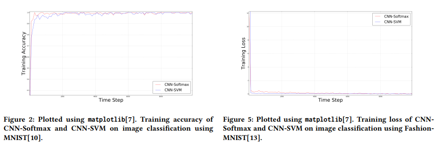
print('Test Accuracy of the model on the 10000 test images: {} %'.format(100 * correct / total))- 밑의 그림은 데이터 분석의 결과표이다.
- Figure2 : CNN-Softmax와 CNN-SVM의 Training Accuracy를 시각화한 표
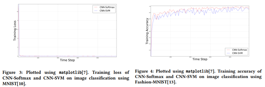
(MNIST) - Figure3 : CNN-Softmax와 CNN-SVM의 Training loss를 시각화한 표
(MNIST) - Figure4 : CNN-Softmax와 CNN-SVM의 Training Accuracy를 시각화한 표
(fashion-MNIST) - Figure5 : CNN-Softmax와 CNN-SVM의 Training loss를 시각화한 표
(fashion-MNIST)
- Figure2 : CNN-Softmax와 CNN-SVM의 Training Accuracy를 시각화한 표
- 모델 성능 (epoch = 10000)
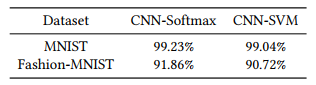
Table 3: Test accuracy of CNN-Softmax and CNN-SVM on image classification using MNIST and Fashion-MNIST
- 직접 구현한 모델 성능 (epoch = 50)
- 학습에 이용한 epoch수가 상이하여 성능에 조금의 차이가 있었지만 다음과 같이 실험환경을 동일하게 구축해볼 수 있었다.
| Dataset | CNN-softmax | CNN-SVM |
|---|---|---|
| MNIST | 98.47% | 98.77% |
| FASHION-MNIST | 88.13% | 87.84% |
4. Conclusion and Rcommendation
-
본 연구 결과는 "Deep Learning using Linear Support Vector Machines"의 제안된 CNN-SVM에 대한 검토를 더욱 검증하기 위한 방법론의 개선을 보증하는데 의의를 둔다.
-
"Deep Learning using Linear Support Vector Machines"의 조사 결과와 모순됨에도 불구하고, 양적으로 말하면, CNN-소프트맥스와 CNN-SVM의 시험 정확도는 관련 연구와 거의 같다.
-
따라서, 추가적인 데이터 사전 처리 및 비교적 정교한 base CNN 모델을 이용하면 충분히 해당 결과를 재현할 수 있을 것이다.