1. Introduction
이번에는 <EDA To Prediction(DieTanic)>이라는 노트북을 공부해보려한다. 이 노트북은 Ashwini Swain이 3년전에 작성한 노트북으로 2021년 1월 4일 기준 128,239의 조회수와 1797개의 투표를 받은 노트북이다.
이 노트북의 큰 틀은 아래와 같다.
Part1: Exploratory Data Analysis(EDA):
- Analysis of the features.

- Finding any relations or trends considering multiple features.
Part2: Feature Engineering and Data Cleaning:
- Adding any few features.

- Removing redundant features.

- Converting features into suitable form for modeling.
Part3: Predictive Modeling
- Running Basic Algorithms.

- Cross Validation.

- Ensembling.

- Important Features Extraction.
2. Part1: Exploratory Data Analysis(EDA)
import numpy as np
import pandas as pd
import matplotlib.pyplot as plt
import seaborn as sns

import warnings
warnings.filterwarnings('ignore')

plt.style.use('fivethirtyeight')
%matplotlib inline
data = pd.read_csv('train.csv')
data.head()| PassengerId | Survived | Pclass | Name | Sex | Age | SibSp | Parch | Ticket | Fare | Cabin | Embarked | |
|---|---|---|---|---|---|---|---|---|---|---|---|---|
| 0 | 1 | 0 | 3 | Braund, Mr. Owen Harris | male | 22.0 | 1 | 0 | A/5 21171 | 7.2500 | NaN | S |
| 1 | 2 | 1 | 1 | Cumings, Mrs. John Bradley (Florence Briggs Th... | female | 38.0 | 1 | 0 | PC 17599 | 71.2833 | C85 | C |
| 2 | 3 | 1 | 3 | Heikkinen, Miss. Laina | female | 26.0 | 0 | 0 | STON/O2. 3101282 | 7.9250 | NaN | S |
| 3 | 4 | 1 | 1 | Futrelle, Mrs. Jacques Heath (Lily May Peel) | female | 35.0 | 1 | 0 | 113803 | 53.1000 | C123 | S |
| 4 | 5 | 0 | 3 | Allen, Mr. William Henry | male | 35.0 | 0 | 0 | 373450 | 8.0500 | NaN | S |
data.isnull().sum()PassengerId 0
Survived 0
Pclass 0
Name 0
Sex 0
Age 177
SibSp 0
Parch 0
Ticket 0
Fare 0
Cabin 687
Embarked 2
dtype: int64Age, Cabin, Embarked 에 Null 값들이 존재하는데 아래에서 수정할 예정이다.
2.1 How many Survived??
f, ax = plt.subplots(1, 2, figsize=(18, 8))
data['Survived'].value_counts().plot.pie(explode=[0, 0.1], autopct='%1.1f%%', ax=ax[0], shadow=True)
ax[0].set_title('Survived')
sns.countplot('Survived', data=data, ax=ax[1])
ax[1].set_title('Survived')
Text(0.5, 1.0, 'Survived')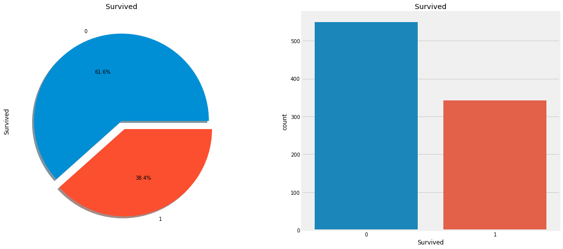
트레인 세트의 891명의 승객 중 350명 즉 38.4%만이 생존하였다. 앞으로 Sex, Embarked, Age 등의 피처로 생존률에 대해 확인해보자.
2.2 Types of Features
- 범주형 피처: Sex, Embarked
범주형 피처는 두 개 혹은 그 이상의 값을 가진 피처로, 예를 들어 성별은 남, 여 이렇게 두가지 피처가 있다. 이런 척도는 명목척도라고도 한다.
- 서열형 피처: Pclass
서열형 피처는 범주형 피처와 유사하지만 그 값들이 상대적 순서가 존재한다. 예를 들어 이 데이터 세트에 있는 Pclass 는 1등석, 2등석, 3등석로 분류 된다.
- 연속형 피처: Age
연속형 피처는 말그대로 숫자가 연속형인 경우이다. 원래는 나이는 28.3세 이런 것은 없지만 이 데이터 세트에는 존재한다.
2.3 Analysing the Features
2.3.1 Sex
data.groupby(['Sex', 'Survived'])['Survived'].count()Sex Survived
female 0 81
1 233
male 0 468
1 109
Name: Survived, dtype: int64f, ax = plt.subplots(1, 2, figsize=(18, 8))
data[['Sex', 'Survived']].groupby(['Sex']).mean().plot.bar(ax=ax[0])
ax[0].set_title('Survived vs Sex')
sns.countplot('Sex', hue='Survived', data=data, ax=ax[1])
ax[1].set_title('Sex: Survived vs Dead')Text(0.5, 1.0, 'Sex: Survived vs Dead')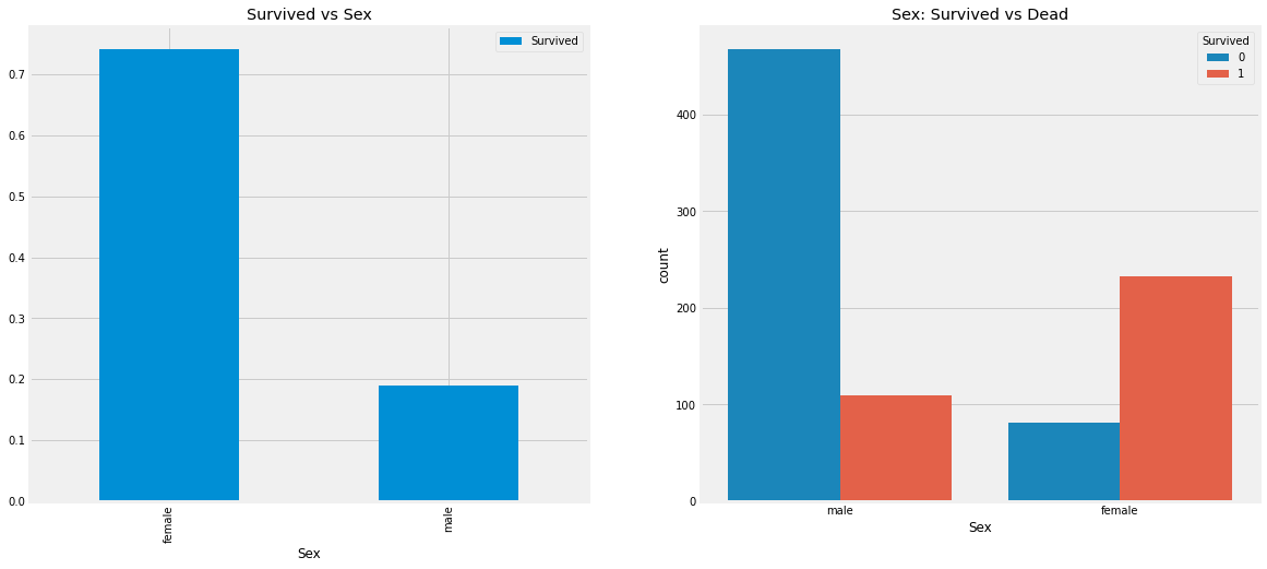
배에 탑승한 남성의 수가 여성의 수보다 훨씬 많지만 여성의 생존률이 남성의 거의 두배이다. 여성의 생존률은 약 75%인 반면, 남성의 생존률은 약 18%이다.
2.3.2 Pclass
pd.crosstab(data.Pclass, data.Survived, margins=True).style.background_gradient(cmap='winter')
f, ax = plt.subplots(1, 2, figsize=(18, 8))
data['Pclass'].value_counts().plot.bar(color=['#CD7F32', '#FFDF00', '#D3D3D3'], ax=ax[0])
ax[0].set_title('Number of Passengers by Pclass')
ax[0].set_ylabel('Count')
sns.countplot('Pclass', hue='Survived', data=data, ax=ax[1])
ax[1].set_title('Pclass: Survived vs Dead')
Text(0.5, 1.0, 'Pclass: Survived vs Dead')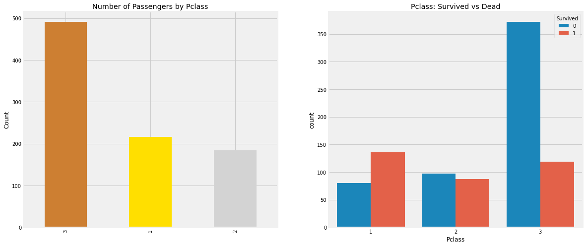
3등급 승객의 수가 더 많은데에 비해 승객의 생존률은 25% 로 매우 낮다. 1등급 승객은 63% 의 생존률, 2등급 승객은 48% 생존률로 등급이 높을수록 높은 생존률을 갖는 것을 알 수 있다.
pd.crosstab([data.Sex, data.Survived], data.Pclass, margins=True).style.background_gradient(cmap='summer_r')
sns.factorplot('Pclass', 'Survived', hue='Sex', data=data)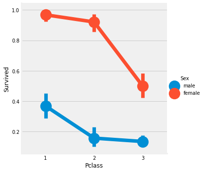
크로스탭 교차표와 요인 분석도를 보면 1등급 여성 94명 중 3명만이 사망했기에 1등급 여성 생존률이 약 95%정도라고 추론할 수 있다. 그리고 Pclass에 관계없이 여성이 남성보다 구조에 우선권이 있었던 것 같다.
2.3.3 Age
print(f'나이가 가장 많은 승객: {data.Age.max()} 살')
print(f'나이가 가장 어린 승객: {data.Age.min()} 살')
print(f'승객들의 평균 나이: {np.round(data.Age.mean(), 2)} 살')
나이가 가장 많은 승객: 80.0 살
나이가 가장 어린 승객: 0.42 살
승객들의 평균 나이: 29.7 살f, ax = plt.subplots(1, 2, figsize=(18, 8))
sns.violinplot('Pclass', 'Age', hue='Survived', data=data, split=True, ax=ax[0])
ax[0].set_title('Pclass & Age vs Survived ')
ax[0].set_yticks(range(0, 110, 10))
sns.violinplot('Sex', 'Age', hue='Survived', data=data, split=True, ax=ax[1])
ax[1].set_title('Sex & Age vs Survived')
ax[1].set_yticks(range(0, 110, 10))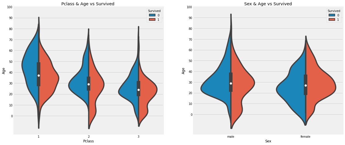
- Pclass 가 1등급에서 3등급으로 갈수록 10세 미만의 승객(어린이)의 수가 증가하며 생존률이 증가한다.
- 1등급 승객중 20-50대 승객의 생존률이 높고 여성의 생존률이 남성보다 높다.
- 남성은 나이가 많을수록 생존률이 줄어든다.
연령에는 177개의 Null 값이 있는데 이는 이름에 있는 Mr, Mrs 등으로 할당할 수 있을거 같다.
data['Initial'] = 0
for i in data:
    data['Initial'] = data.Name.str.extract('([A-Za-z]+)\.')

pd.crosstab(data.Sex, data.Initial).style.background_gradient(cmap='summer_r')
Initial 의 범주가 너무 많으므로 대부분을 차지하는 Miss, Mr, Mrs 등으로 대체한다.
- Mile, Mme, Ms -> Miss
- Dr, Major, Capt, Sir, Don -> Mr
- Lady, Countess -> Mrs
- Jonkheer, Col, Rev -> Other
사실 난 여기서 Jonkheer, Col, Rev를 남자로 바꿨으면 어땠을까 생각이 든다. 비교를 위해 한번 내 생각대로 진행해보려한다. 원본대로 하는 것은 깃허브에 올려두었다.
data['Initial'].replace(['Mlle','Mme','Ms','Dr','Major','Lady','Countess','Jonkheer','Col','Rev','Capt','Sir','Don'], ['Miss','Miss','Miss','Mr','Mr','Mrs','Mrs','Mr','Mr','Mr','Mr','Mr','Mr'],inplace=True)data.groupby('Initial')['Age'].mean()Initial
Master 4.574167
Miss 21.860000
Mr 33.022727
Mrs 35.981818
Name: Age, dtype: float64Filling NaN Ages
위에서 Initial 각각의 평균 나이로 나이의 Null 값을 채운다.
Master: 5, Miss: 22, Mr: 33, Mrs: 36
data.loc[(data.Age.isnull()) & (data.Initial == 'Master'), 'Age'] = 5
data.loc[(data.Age.isnull()) & (data.Initial == 'Miss'), 'Age'] = 22
data.loc[(data.Age.isnull()) & (data.Initial == 'Mr'), 'Age'] = 33
data.loc[(data.Age.isnull()) & (data.Initial == 'Mrs'), 'Age'] = 36data.Age.isnull().any()Falsef, ax = plt.subplots(1, 2, figsize=(20, 10))
data[data['Survived']==0].Age.plot.hist(ax=ax[0], bins=20, edgecolor='black', color='red')
ax[0].set_title('Survived = 0')
x1 = list(range(0, 85, 5))
ax[0].set_xticks(x1)
data[data['Survived']==1].Age.plot.hist(ax=ax[1], bins=20, edgecolor='black', color='green')
ax[1].set_title('Survived = 1')
ax[1].set_xticks(x1)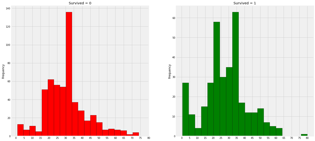
- 0-5세 어린이의 생존률이 매우 높다.
- 최고령 생존 승객은 80세이다.
- 사망자가 많은 나이는 30-35세이다.
sns.factorplot('Pclass', 'Survived', col='Initial', data=data)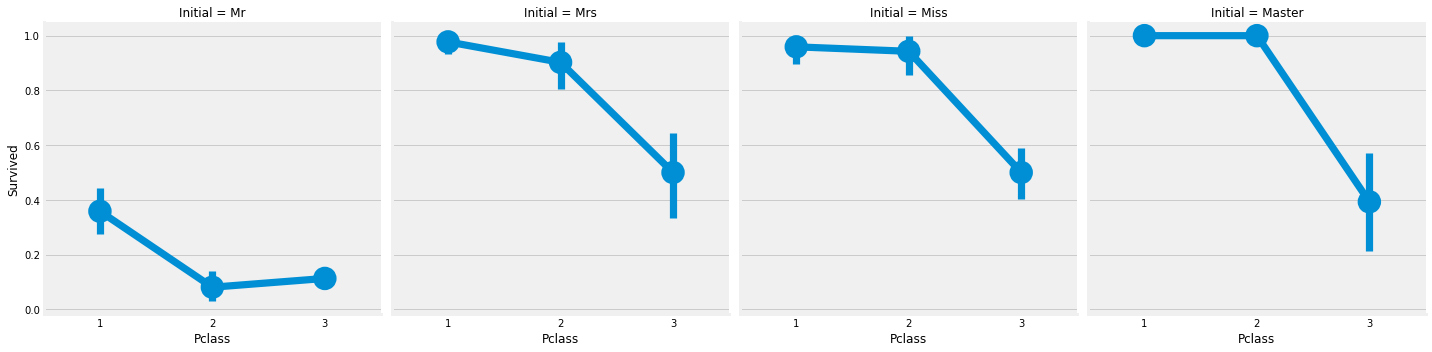
2.3.4 Embarked
pd.crosstab([data.Embarked, data.Pclass], [data.Sex, data.Survived], margins=True).style.background_gradient(cmap='summer_r')
sns.factorplot('Embarked', 'Survived', data=data)
fig = plt.gcf()
fig.set_size_inches(5, 3)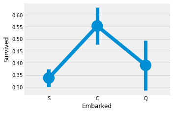
C 에서 탑승한 승객의 생존률이 약 55% 정도로 나타나고 S 에서 탑승한 승객의 생존률이 가장 낮게 나타난다.
f, ax = plt.subplots(2, 2, figsize=(20, 15))
sns.countplot('Embarked', data=data, ax=ax[0,0])
ax[0,0].set_title('No. of Passengers Boarded')
sns.countplot('Embarked', hue='Sex', data=data, ax=ax[0,1])
ax[0,1].set_title('Male-Female Split for Embarked')
sns.countplot('Embarked', hue='Survived', data=data, ax=ax[1,0])
ax[1,0].set_title('Embarked vs Survived')
sns.countplot('Embarked', hue='Pclass', data=data, ax=ax[1,1])
ax[1,1].set_title('Embarked vs Pclass')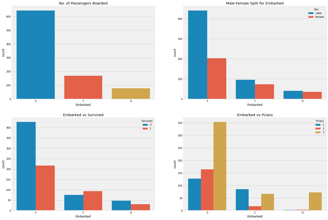
- S에서 탑승한 승객의 수가 가장 많고 그들은 대부분 3등급 승객이다.
- C에서 탑승한 승객의 생존률이 높은 이유는 아마 그들이 1등급 승객이 많아서일 것이다.
- Q에서 탑승한 승객의 대부분은 3등급 승객이다.
sns.factorplot('Pclass', 'Survived', hue='Sex', col='Embarked', data=data)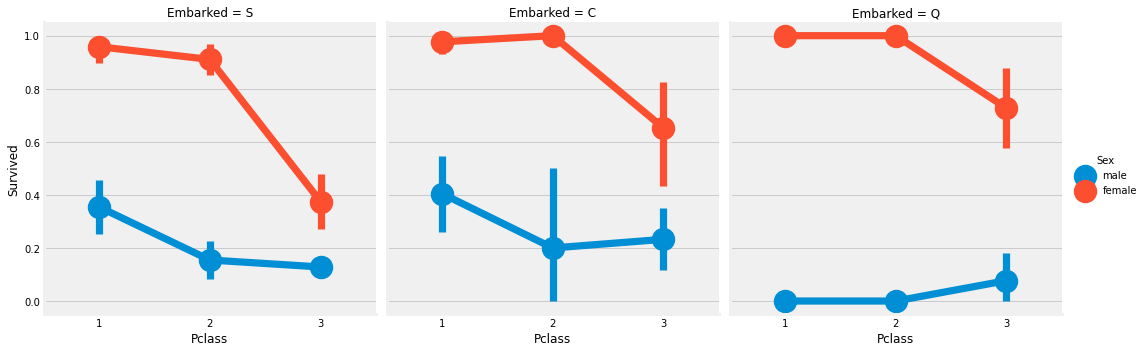
- Pclass 가 1등급, 2등급 인 경우 여성의 생존률은 1에 근사하다.
- S 에서 탑승한 3등급 승객은 남녀 구분없이 생존률이 낮다.
- Q 에서 탑승한 승객은 대부분 3등급 승객이여서 남성의 생존률이 낮게 나타난다.
Filling Embarked NaN
대부분 승객이 S 에서 탑승했으므로 Null 값을 모두 S 로 대체한다.
data['Embarked'].fillna('S', inplace=True)
data.Embarked.isnull().any()False2.3.5 SibSp
pd.crosstab(data.Survived, data.SibSp).style.background_gradient(cmap='summer_r')
sns.barplot('SibSp', 'Survived', data=data)
plt.title('SibSp vs Survived')
sns.factorplot('SibSp', 'Survived', data=data)
plt.title('SibSp vs Survived')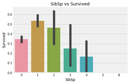
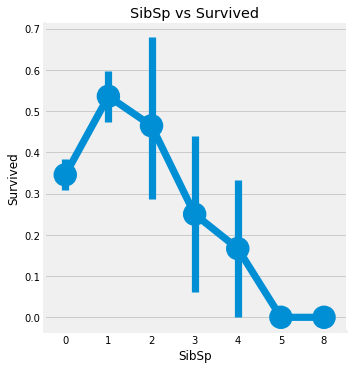
pd.crosstab(data.Pclass, data.SibSp).style.background_gradient(cmap='summer_r')
혼자 탑승한 경우 생존률은 약 34.5% 정도이고 형제/자매/배우자의 수가 1, 2명일때가 3명 이상일때보다 생존률이 높다. 5-8명의 형제/자매/배우자를 가진 사람의 생존률이 0%인 이유는 Pclass의 영향으로 보인다. 크로스탭 교차표에 따르면 모두 3등급 승객임을 알 수 있다.
2.3.6 Parch
pd.crosstab(data.Pclass, data.Parch).style.background_gradient(cmap='summer_r')
sns.barplot('Parch', 'Survived', data=data)
plt.title('Parch vs Survived')
sns.factorplot('Parch', 'Survived', data=data)
plt.title('Parch vs Survived')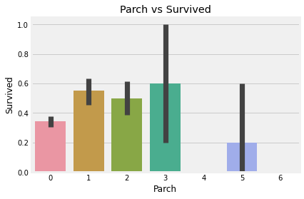
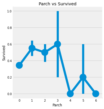
부모/자식이 1-3명인 승객의 생존률이 혼자 탑승했거나 4-6명인 승객의 생존률보다 높다. 위에 SibSp의 경우와 유사하다.
2.3.7 Fare
print(f'가장 비싼 요금: {data.Fare.max()}')
print(f'가장 싼 요금: {data.Fare.min()}')
print(f'요금의 평균: {np.round(data.Fare.mean(), 4)}')
가장 비싼 요금: 512.3292
가장 싼 요금: 0.0
요금의 평균: 32.2042f, ax = plt.subplots(1, 3, figsize=(20, 8))
for i in range(3):
sns.distplot(data[data['Pclass']==i+1].Fare, ax=ax[i])
ax[i].set_title(f'Fare in Pclass {i+1}')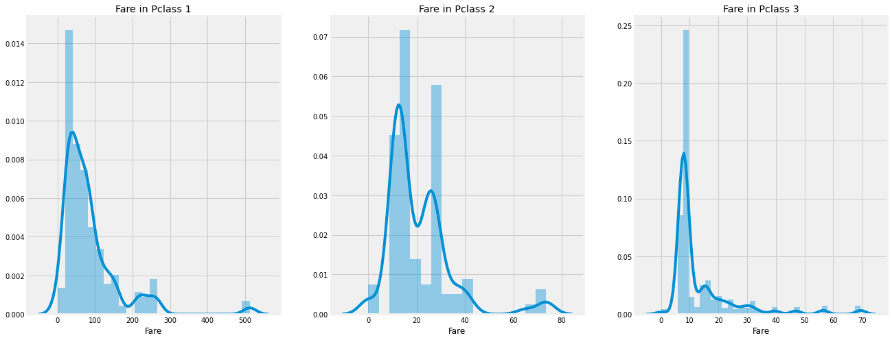
확실히 1등급의 요금이 2, 3등급보다 비싼 것을 알 수 있다.
2.4 Observations in NutShell for all Features
- Sex: 여성의 생존률이 남성보다 높다.
- Pclass: 1등급의 생존률이 거의 1에 수렴하며 2등급의 생존률이 높고 3등급의 생존률이 낮다.
- Age: 10세 미만의 어린이들의 생존률이 높고 15-35세의 승객들의 사망률이 높다.
- Embarked: 1등급 승객이 많은 C에서 탑승한 승객의 생존률이 가장 높다.
- Parch & SibSp: 1-2명의 형제/자매가 있거나 1-3명의 부모/자식이 있는 승객의 생존률이 혼자거나 대가족인 경우보다 높다.
3. Part2: Feature Engineering and Data Cleaning
3.1 Feature Engineering
3.1.1 Age_band
Age 는 연속형 변수인데 연속형 변수는 ML 모델에 영향을 준다. 그래서 카테고리형 변수로 변환해주어야하는데 가장 나이가 많은 승객이 80살이였으니 이를 5개 구간 즉 16살 단위로 나누어 볼 수 있다.
data['Age_band'] = 0
data.loc[data['Age']<=16, 'Age_band'] = 0
data.loc[(data['Age']>16) & (data['Age']<=32), 'Age_band'] = 1
data.loc[(data['Age']>32) & (data['Age']<=48), 'Age_band'] = 2
data.loc[(data['Age']>48) & (data['Age']<=64), 'Age_band'] = 3
data.loc[data['Age']>64, 'Age_band'] = 4
data.head(2)| PassengerId | Survived | Pclass | Name | Sex | Age | SibSp | Parch | Ticket | Fare | Cabin | Embarked | Initial | Age_band | |
|---|---|---|---|---|---|---|---|---|---|---|---|---|---|---|
| 0 | 1 | 0 | 3 | Braund, Mr. Owen Harris | male | 22.0 | 1 | 0 | A/5 21171 | 7.2500 | NaN | S | Mr | 1 |
| 1 | 2 | 1 | 1 | Cumings, Mrs. John Bradley (Florence Briggs Th... | female | 38.0 | 1 | 0 | PC 17599 | 71.2833 | C85 | C | Mrs | 2 |
data['Age_band'].value_counts().to_frame().style.background_gradient(cmap='summer_r')
sns.factorplot('Age_band', 'Survived', col='Pclass',data=data)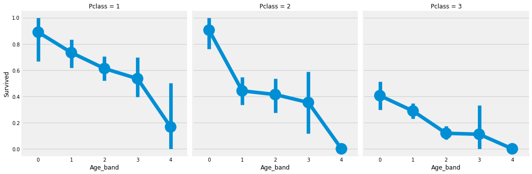
Pclass에 관계없이 나이가 증가함에 따라 생존률은 감소한다.
3.1.2 Family_Size and Alone
Family_Size 는 Parch 와 SibSp 를 이용해서 만들 수 있다.
data['Family_Size'] = 0
data['Alone'] = 0
data['Family_Size'] = data['Parch'] + data['SibSp'] + 1
data.loc[data.Family_Size==1, 'Alone'] = 1

sns.factorplot('Family_Size', 'Survived', data=data)
plt.title('Family_Size vs Survived')
sns.factorplot('Alone', 'Survived', data=data)
plt.title('Alone vs Survived')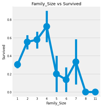
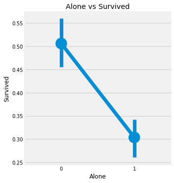
Family_Size = 1 은 혼자 탑승한 승객을 의미하며, 혼자 탑승한 승객과 Family_Size 가 4보다 큰 경우의 생존률이 저조한 것을 알 수 있다.
sns.factorplot('Alone', 'Survived', data=data, hue='Sex', col='Pclass')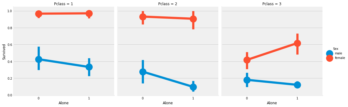
1등급, 3등급 여성 승객의 경우를 제외하고 혼자 탑승한 경우의 생존률이 더 낮게 나타난다.
3.1.3 Fare_Range
Fare 역시 연속형 변수로 이번엔 pandas.qcut을 이용해서 4개의 범위로 나누어보자.
data['Fare_range'] = pd.qcut(data['Fare'], 4)
data.groupby(['Fare_range'])['Survived'].mean().to_frame().style.background_gradient(cmap='summer_r')
요금이 증가함에따라 생존률도 증가하는 것을 알 수 있다. 이대로 ML 모델에 적용할 수 없으니 Age_Band 처럼 인코딩 해줘야한다.
data['Fare_cat'] = 0
data.loc[data['Fare']<=7.91,'Fare_cat'] = 0
data.loc[(data['Fare']>7.91)&(data['Fare']<=14.454),'Fare_cat'] = 1
data.loc[(data['Fare']>14.454)&(data['Fare']<=31),'Fare_cat'] = 2
data.loc[(data['Fare']>31)&(data['Fare']<=513),'Fare_cat'] = 3

sns.factorplot('Fare_cat', 'Survived', data=data, hue='Sex')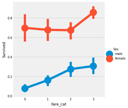
3.1.4 Converting String Values into Numeric
문자형인 Sex, Embarked, Initial 에 대해 매핑을 진행하자.
data['Sex'].replace(['male', 'female'], [0, 1], inplace=True)
data['Embarked'].replace(['S', 'C', 'Q'], [0, 1, 2], inplace=True)
data['Initial'].replace(['Mr', 'Mrs', 'Miss', 'Master', 'Other'], [0, 1, 2, 3, 4], inplace=True)
3.2 Dropping UnNeeded Features
data.drop(['Name', 'Age', 'Ticket', 'Fare', 'Cabin', 'Fare_range', 'PassengerId'], axis=1, inplace=True)

sns.heatmap(data.corr(), annot=True, cmap='RdYlGn', linewidths=0.2, annot_kws={'size':20})
fig = plt.gcf()
fig.set_size_inches(18, 15)
plt.xticks(fontsize=14)
plt.yticks(fontsize=14)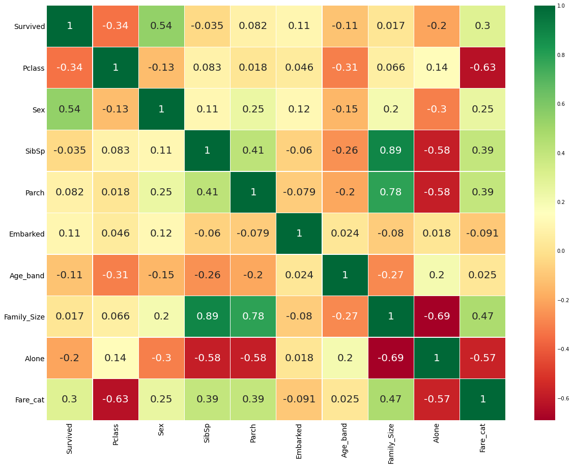
4. Part3: Predictive Modeling
4.1 ML Algorithm
사용할 알고리즘:
1. Logistic Regression
2. Support Vector Machines(Linear and radial)
3. Random Forest
4. K-Nearest Neighbours
5. Naive Bayes
6. Decision Tree
from sklearn.linear_model import LogisticRegression
from sklearn import svm
from sklearn.ensemble import RandomForestClassifier
from sklearn.neighbors import KNeighborsClassifier
from sklearn.naive_bayes import GaussianNB
from sklearn.tree import DecisionTreeClassifier
from sklearn.model_selection import train_test_split
from sklearn import metrics
from sklearn.metrics import confusion_matrixtrain, test = train_test_split(data, test_size=0.3, random_state=0, stratify=data['Survived'])
train_X = train[train.columns[1:]]
train_Y = train[train.columns[:1]]
test_X = test[test.columns[1:]]
test_Y = test[test.columns[:1]]
X = data[data.columns[1:]]
Y = data['Survived']4.1.1 Radial Support Vector Machines(rbf-SVM)
model = svm.SVC(kernel='rbf', gamma=0.1)
model.fit(train_X, train_Y)
prediction1 = model.predict(test_X)
print(f'Accuracy of the rbf SVM: {metrics.accuracy_score(prediction1, test_Y)}')
Accuracy of the rbf SVM: 0.8358208955223884.1.2 Linear Support Vector Machines(linear-SVM)
model = svm.SVC(kernel='linear', C=0.1, gamma=0.1)
model.fit(train_X, train_Y)
prediction2 = model.predict(test_X)
print(f'Accuracy of the linear SVM: {metrics.accuracy_score(prediction2, test_Y)}')
Accuracy of the linear SVM: 0.81716417910447764.1.3 Logistic Regression
model = LogisticRegression()
model.fit(train_X, train_Y)
prediction3 = model.predict(test_X)
print(f'Accuracy of the Logistic Regression: {metrics.accuracy_score(prediction3, test_Y)} ')
Accuracy of the Logistic Regression: 0.8171641791044776 4.1.4 Decision Tree
model = DecisionTreeClassifier()
model.fit(train_X, train_Y)
prediction4 = model.predict(test_X)
print(f'Accuracy of the Decision Tree: {metrics.accuracy_score(prediction4, test_Y)}')
Accuracy of the Decision Tree: 0.80223880597014934.1.5 K-Nearest Neighbors(KNN)
model = KNeighborsClassifier()
model.fit(train_X, train_Y)
prediction5 = model.predict(test_X)
print(f'Accuracy of the KNN: {metrics.accuracy_score(prediction5, test_Y)}')
Accuracy of the KNN: 0.8246268656716418KNN 모델의 n_neighbors 값의 디폴트 값은 5이다. 이 값을 0부터 10까지 변화 시키면서 확인해보자.
x = list(range(1, 11))
a = pd.Series()
for i in x:
    model = KNeighborsClassifier(n_neighbors=i)
    model.fit(train_X, train_Y)
    prediction = model.predict(test_X)
    a = a.append(pd.Series(metrics.accuracy_score(prediction, test_Y)))
plt.plot(x, a)
plt.xticks(x)
fig=plt.gcf()
fig.set_size_inches(12, 6)
print(f'Accuracies of different values of n are:\n {a.values} \nwith the max value as {a.values.max()}')
Accuracies of different values of n are:
[0.77985075 0.79850746 0.79850746 0.78731343 0.82462687 0.80597015
0.82089552 0.81716418 0.83208955 0.82089552]
with the max value as 0.832089552238806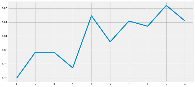
4.1.6 Gaussian Naive Bayes
model = GaussianNB()
model.fit(train_X, train_Y)
prediction6 = model.predict(test_X)
print(f'Accuracy of the Naive Bayes: {metrics.accuracy_score(prediction6, test_Y)}')
Accuracy of the Naive Bayes: 0.81343283582089554.1.7 Random Forest
model = RandomForestClassifier(n_estimators=100)
model.fit(train_X, train_Y)
prediction7 = model.predict(test_X)
print(f'Accuracy of the Random Forest: {metrics.accuracy_score(prediction7, test_Y)}')
Accuracy of the Random Forest: 0.81716417910447764.1.8 K-fold Cross Validation
from sklearn.model_selection import KFold
from sklearn.model_selection import cross_val_predict, cross_val_score

kfold = KFold(n_splits=10, random_state=22)
xyz = []
accuracy = []
std = []
classifiers = ['Linear SVM', 'Radial SVM', 'Logistic Regression', 'KNN', 'Decision Tree', 'Naive Bayes', 'Random Forest']
models = [svm.SVC(kernel='linear'), svm.SVC(kernel='rbf'), LogisticRegression(), KNeighborsClassifier(n_neighbors=9), DecisionTreeClassifier(), GaussianNB(), RandomForestClassifier(n_estimators=100)]

for i in models:
    model = i
    cv_result = cross_val_score(model, X, Y, cv=kfold, scoring='accuracy')
    xyz.append(cv_result.mean())
    std.append(cv_result.std())
    accuracy.append(cv_result)
new_models_dataframe2 = pd.DataFrame({'CV Mean': xyz, 'std': std}, index=classifiers)
new_models_dataframe2| CV Mean | std | |
|---|---|---|
| Linear SVM | 0.820437 | 0.042882 |
| Radial SVM | 0.829413 | 0.034694 |
| Logistic Regression | 0.818202 | 0.023813 |
| KNN | 0.809288 | 0.035233 |
| Decision Tree | 0.808115 | 0.031311 |
| Naive Bayes | 0.811498 | 0.029233 |
| Random Forest | 0.820474 | 0.032227 |
plt.subplots(figsize=(12, 6))
box = pd.DataFrame(accuracy, index=[classifiers])
box.T.boxplot()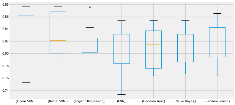
new_models_dataframe2['CV Mean'].plot.barh(width=0.8)
plt.title('Average CV Mean Accuracy')
fig = plt.gcf()
fig.set_size_inches(8, 5)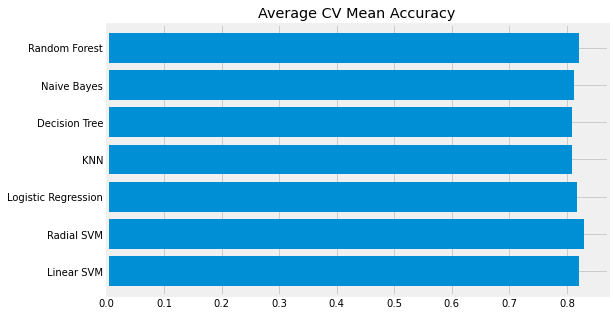
정확도는 불균형한 레이블 데이터 세트에서는 성능 수치로 사용되어서는 안되기에 오차행렬을 통해 모델의 성능을 확인해 볼 수 있다.
4.2 Confusion Matrix
f, ax = plt.subplots(3, 3, figsize=(12, 10))
y_pred = cross_val_predict(svm.SVC(kernel='rbf'), X, Y, cv=10)
sns.heatmap(confusion_matrix(Y, y_pred), ax=ax[0,0], annot=True, fmt='2.0f')
ax[0,0].set_title('Matrix for rbf-SVM')
y_pred = cross_val_predict(svm.SVC(kernel='linear'), X, Y, cv=10)
sns.heatmap(confusion_matrix(Y, y_pred), ax=ax[0,1], annot=True, fmt='2.0f')
ax[0,1].set_title('Matrix for Linear-SVM')
y_pred = cross_val_predict(KNeighborsClassifier(n_neighbors=9),X,Y,cv=10)
sns.heatmap(confusion_matrix(Y,y_pred),ax=ax[0,2],annot=True,fmt='2.0f')
ax[0,2].set_title('Matrix for KNN')
y_pred = cross_val_predict(RandomForestClassifier(n_estimators=100),X,Y,cv=10)
sns.heatmap(confusion_matrix(Y,y_pred),ax=ax[1,0],annot=True,fmt='2.0f')
ax[1,0].set_title('Matrix for Random-Forests')
y_pred = cross_val_predict(LogisticRegression(),X,Y,cv=10)
sns.heatmap(confusion_matrix(Y,y_pred),ax=ax[1,1],annot=True,fmt='2.0f')
ax[1,1].set_title('Matrix for Logistic Regression')
y_pred = cross_val_predict(DecisionTreeClassifier(),X,Y,cv=10)
sns.heatmap(confusion_matrix(Y,y_pred),ax=ax[1,2],annot=True,fmt='2.0f')
ax[1,2].set_title('Matrix for Decision Tree')
y_pred = cross_val_predict(GaussianNB(),X,Y,cv=10)
sns.heatmap(confusion_matrix(Y,y_pred),ax=ax[2,0],annot=True,fmt='2.0f')
ax[2,0].set_title('Matrix for Naive Bayes')
plt.subplots_adjust(hspace=0.2,wspace=0.2)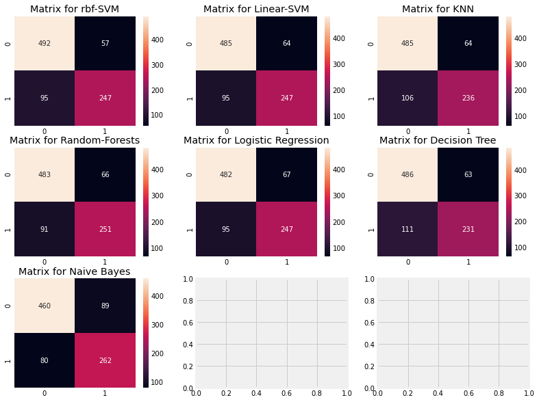
- 예측
첫 번째 그림을 보면 82.8% 정확도로 예측한 것을 알 수 있다. - 오류
58명의 사망자를 생존자로 잘못 분류되었고, 95명의 생존자를 사망자로 잘못 분류하였다.
rbf-SVM 은 사망자(492명)에 대해 제일 정확하게 예측했고, Naive Bayes 는 생존자(262명)에 대해 제일 정확하게 예측했다.
4.3 Hyper-Parameters Tuning
SVM과 Random Forest의 하이퍼 파라미터를 찾아보자.
4.3.1 SVM
from sklearn.model_selection import GridSearchCV
C = [0.05, 0.1, 0.2, 0.3, 0.4, 0.5, 0.6, 0.7, 0.8, 0.9, 1]
gamma = [0.1, 0.2, 0.3, 0.4, 0.5, 0.6, 0.7, 0.8, 0.9, 1]
kernel = ['rbf', 'linear']
hyper = {'kernel': kernel, 'C': C, 'gamma': gamma}
gd = GridSearchCV(estimator=svm.SVC(), param_grid=hyper, verbose=True)
gd.fit(X, Y)
print(gd.best_score_)
print(gd.best_params_)
Fitting 5 folds for each of 220 candidates, totalling 1100 fits
[Parallel(n_jobs=1)]: Using backend SequentialBackend with 1 concurrent workers.
0.8293829640323898
{'C': 0.6, 'gamma': 0.1, 'kernel': 'rbf'}
[Parallel(n_jobs=1)]: Done 1100 out of 1100 | elapsed: 16.3s finished4.3.2 Random Forest
n_estimators = range(100, 1000, 100)
hyper = {'n_estimators': n_estimators}
gd = GridSearchCV(estimator=RandomForestClassifier(random_state=0), param_grid=hyper, verbose=True)
gd.fit(X, Y)
print(gd.best_score_)
print(gd.best_params_)
[Parallel(n_jobs=1)]: Using backend SequentialBackend with 1 concurrent workers.
Fitting 5 folds for each of 9 candidates, totalling 45 fits
[Parallel(n_jobs=1)]: Done 45 out of 45 | elapsed: 30.8s finished
0.8193270981106021
{'n_estimators': 900}SVM은 {'C': 0.6, 'gamma': 0.1, 'kernel': 'rbf'} 에서 82.94% 정확도를 보였고, RandomForest는 {'n_estimators': 900} 에서 81.93% 의 정확도를 보였다.
4.4 Ensembling
앙상블 기법으로는 다음과 같은 방법이 있다.
- Voting
- Bagging
- Boosting
4.4.1 Voting Classifier
여러 개의 ML 모델의 예측을 결합하는 가장 간단한 방법으로 모든 하위 모델의 예측에 기반한 평균 예측 결과를 제공한다.
from sklearn.ensemble import VotingClassifier
ensemble_lin_rbf = VotingClassifier(estimators=[('KNN', KNeighborsClassifier(n_neighbors=10)),
                                               ('RBF', svm.SVC(probability=True, kernel='rbf', C=0.6, gamma=0.1)),
                                               ('RFor', RandomForestClassifier(n_estimators=900, random_state=0)),
                                               ('LR', LogisticRegression(C=0.05)),
                                               ('DT', DecisionTreeClassifier(random_state=0)),
                                               ('NB', GaussianNB()),
                                               ('svm', svm.SVC(kernel='linear', probability=True))
                                               ], voting='soft').fit(train_X, train_Y)
print(f'The Accuracy for Ensembled Model is: {ensemble_lin_rbf.score(test_X, test_Y)}')
cross = cross_val_score(ensemble_lin_rbf, X, Y, cv=10, scoring='accuracy')
print(f'The cross validated score is: {cross.mean()}')
The Accuracy for Ensembled Model is: 0.8208955223880597
The cross validated score is: 0.82604244694132344.4.2 Bagging
배깅은 샘플을 여러번 뽑아 각 모델을 학습시켜 결과를 집계하는 방법이다. 배깅은 분산이 높은 모형에서 가장 적합하다. 이는 KNN 과 Decision Tree 에서 적용해 볼 수 있다.
KNN
from sklearn.ensemble import BaggingClassifier
model = BaggingClassifier(base_estimator=KNeighborsClassifier(n_neighbors=3), random_state=0, n_estimators=700)
model.fit(train_X, train_Y)
prediction = model.predict(test_X)
print(f'The Accuracy for Bagged KNN: {metrics.accuracy_score(prediction, test_Y)}')
result = cross_val_score(model, X, Y, cv=10, scoring='accuracy')
print(f'The cross validated score is: {result.mean()}')
The Accuracy for Bagged KNN: 0.832089552238806
The cross validated score is: 0.8137952559300873Decision Tree
model = BaggingClassifier(base_estimator=DecisionTreeClassifier(), random_state=0, n_estimators=100)
model.fit(train_X, train_Y)
prediction = model.predict(test_X)
print(f'The Accuracy for Bagged Decision Tree: {metrics.accuracy_score(prediction, test_Y)}')
result = cross_val_score(model, X, Y, cv=10, scoring='accuracy')
print(f'The cross validated score is: {result.mean()}')
The Accuracy for Bagged Decision Tree: 0.8283582089552238
The cross validated score is: 0.81489388264669174.4.3 Boosting
배깅이 일반적인 모델을 만드는데 집중되어있다면, 부스팅은 맞추기 어려운 문제를 맞추는데 초점이 맞춰져있다. 즉, 전체 데이터 집합에 대해 교육을 한 후, 다음 반복에서 잘못 예측된 사례에 더 집중하거나 비중을 두어 잘못 예측된 인스턴스를 올바르게 예측하려고 시도한다.
AdaBoost
from sklearn.ensemble import AdaBoostClassifier
ada = AdaBoostClassifier(n_estimators=200, random_state=0, learning_rate=0.1)
result = cross_val_score(ada, X, Y, cv=10, scoring='accuracy')
print(f'The cross validated score for AdaBoost is: {result.mean()}')
The cross validated score for AdaBoost is: 0.8226716604244695Strochastic Gradient Boosting(경사하강법)
from sklearn.ensemble import GradientBoostingClassifier
grad = GradientBoostingClassifier(n_estimators=500, random_state=0, learning_rate=0.1)
result = cross_val_score(grad, X, Y, cv=10, scoring='accuracy')
print(f'The cross validated score for Gradient Boosting is: {result.mean()}')
The cross validated score for Gradient Boosting is: 0.8137952559300874XGBoost
import xgboost as xg
xgboost = xg.XGBClassifier(n_estimators=900, learning_rate=0.1)
result = cross_val_score(xgboost, X, Y, cv=10, scoring='accuracy')
print(f'The cross validated score for XGBoost is: {result.mean()}')
The cross validated score for XGBoost is: 0.8160299625468165AdaBoost의 정확도가 가장 높으므로 AdaBoost에 대해 하이퍼 파라미터 튜닝을 진행한다.
n_estimators = list(range(100, 1100, 100))
learn_rate = [0.05, 0.1, 0.2, 0.25, 0.3, 0.4, 0.5, 0.6, 0.7, 0.8, 0.9, 1.0]
hyper = {'n_estimators': n_estimators,
        'learning_rate': learn_rate}
gd = GridSearchCV(estimator=AdaBoostClassifier(), param_grid=hyper, verbose=True)
gd.fit(X, Y)
print(gd.best_score_)
print(gd.best_estimator_)
Fitting 5 folds for each of 120 candidates, totalling 600 fits
[Parallel(n_jobs=1)]: Using backend SequentialBackend with 1 concurrent workers.
0.8316238779737619
AdaBoostClassifier(learning_rate=0.05, n_estimators=100)
[Parallel(n_jobs=1)]: Done 600 out of 600 | elapsed: 9.9min finishedAdaBoost의 정확도는 82.94% 이고 최고의 파라미터는 n_estimators=100, learning_rate=0.1 이다.
4.5 Confusion Matrix for the Best Model
ada = AdaBoostClassifier(n_estimators=100, random_state=0, learning_rate=0.1)
result = cross_val_predict(ada, X, Y, cv=10)
sns.heatmap(confusion_matrix(Y, result), cmap='winter', annot=True, fmt='2.0f')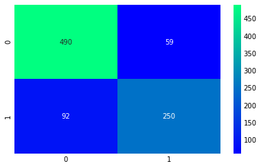
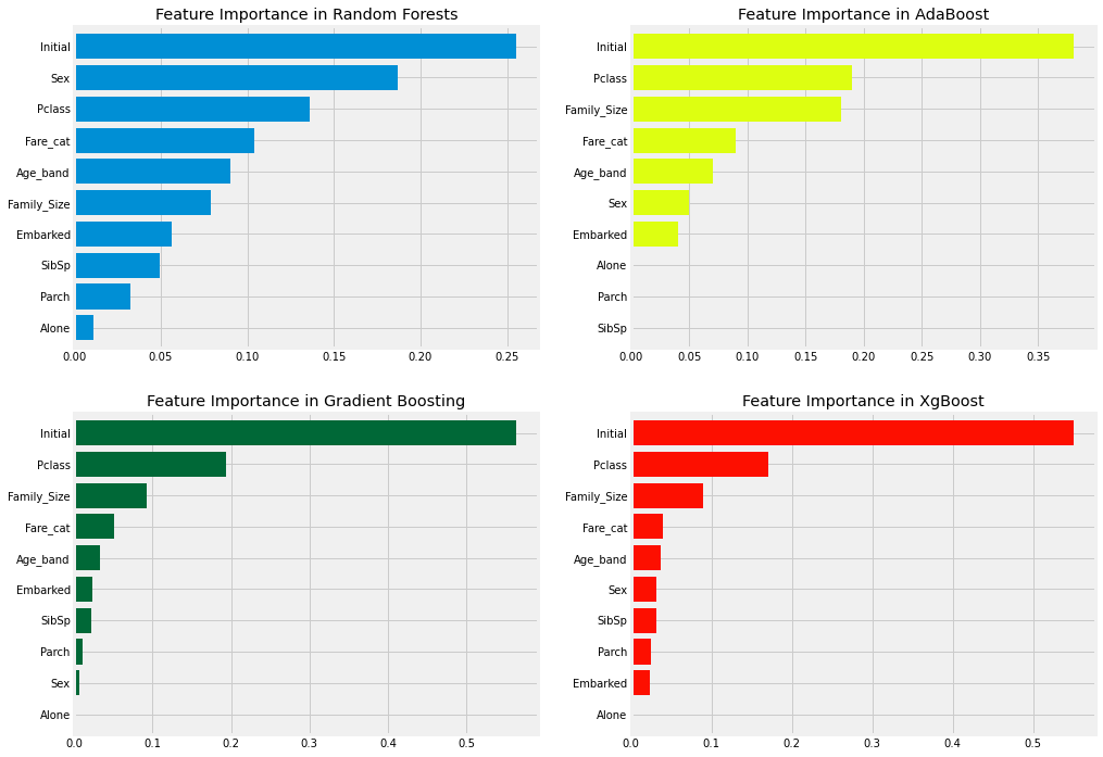
4.6 Feature Importance
f, ax = plt.subplots(2, 2, figsize=(15, 12))
model = RandomForestClassifier(n_estimators=300, random_state=0)
model.fit(X, Y)
pd.Series(model.feature_importances_, X.columns).sort_values(ascending=True).plot.barh(width=0.8, ax=ax[0,0])
ax[0,0].set_title('Feature Importance in Random Forests')
model = AdaBoostClassifier(n_estimators=100, learning_rate=0.1, random_state=0)
model.fit(X, Y)
pd.Series(model.feature_importances_, X.columns).sort_values(ascending=True).plot.barh(width=0.8, ax=ax[0,1], color='#ddff11')
ax[0,1].set_title('Feature Importance in AdaBoost')
model = GradientBoostingClassifier(n_estimators=500, learning_rate=0.1, random_state=0)
model.fit(X, Y)
pd.Series(model.feature_importances_, X.columns).sort_values(ascending=True).plot.barh(width=0.8, ax=ax[1,0], cmap='RdYlGn_r')
ax[1,0].set_title('Feature Importance in Gradient Boosting')
model = xg.XGBClassifier(n_estimators=900, learning_rate=0.1)
model.fit(X, Y)
pd.Series(model.feature_importances_, X.columns).sort_values(ascending=True).plot.barh(width=0.8, ax=ax[1,1], color='#FD0F00')
ax[1,1].set_title('Feature Importance in XgBoost')