피마 인디언 당뇨병 예측 데이터 세트로 머신러닝 평가하기

이번에는 Kaggle의 피마 인디언 당뇨병(Pima Indian Diabetes) 데이터 세트를 이용해 당뇨병 여부를 판단하는 머신러닝 예측 모델을 수립하고, 저번에 작성한 평가 지표를 적용해 보자.

Kaggle: Pima Indian Diabetes 데이터 세트

1. 데이터 세트 확인

피마 인디언 당뇨병 데이터 세트는 아래와 같이 구성되어있다.

• Pregnancies: 임신 횟수
• Glucose: 포도당 부하 검사 수치
• BloodPressure: 혈압(mm Hg)
• SkinThickness: 팔 삼두근 뒤쪽의 피하지방 측정값(mm)
• Insulin: 혈청 인슐린(mu U/ml)
• BMI: 체질량지수(체중(kg)/키(m))^2
• DiabetesPedigreeFunction: 당뇨 내력 가중치 값
• Age: 나이
• Outcome: 클래스 결정 값(0 또는 1)

import numpy as np
import pandas as pd
import matplotlib.pyplot as plt
%matplotlib inline

from sklearn.model_selection import train_test_split
from sklearn.metrics import accuracy_score, precision_score, recall_score, roc_auc_score
from sklearn.metrics import f1_score, confusion_matrix, precision_recall_curve, roc_curve
from sklearn.preprocessing import StandardScaler, Binarizer
from sklearn.linear_model import LogisticRegression

import warnings
warnings.filterwarnings('ignore')

diabetes_data = pd.read_csv('diabetes.csv')
print(diabetes_data['Outcome'].value_counts())
diabetes_data.head(5)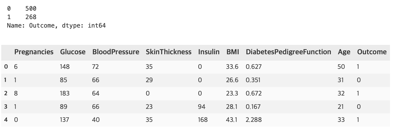

768개의 데이터 중 Negative 값(0)이 500개, Positive 값(1)이 268개로 Negative가 상대적으로 많다. 즉, 전체 데이터의 65.1%가 Negative이다.

diabetes_data.info()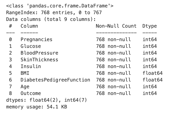

Titanic과 다르게 Null 값은 없고 피처의 타입이 모두 숫자형이므로 별도의 피처 인코딩은 필요하지 않아 보인다.

2. 유틸리티 함수 생성

저번에 사용한 유틸리티 함수 get_clf_eval(), get_eval_by_threshold(), precision_recall_curve_plot()을 이용하려하니 저번 함수들을 가져온다.

# get_clf_eval()
# 저번에 작성한 것에 ROC AUC를 추가함
def get_clf_eval(y_test, pred=None, pred_proba=None):
    confusion = confusion_matrix(y_test, pred)
    accuracy = accuracy_score(y_test, pred)
    precision = precision_score(y_test, pred)
    recall = recall_score(y_test, pred)
    f1 = f1_score(y_test, pred)
    roc_auc = roc_auc_score(y_test, pred)
    
    print('오차행렬')
    print(confusion)
    print('정확도: {0:.4f}, 정밀도: {1:.4f}, 재현율: {2:.4f}, F1: {3:.4f}, AUC:{4:.4f}'
          .format(accuracy, precision, recall, f1, roc_auc))
    
# get_eval_by_threshold()
def get_eval_by_threshold(y_test, pred_proba_c1, thresholds):
    # thresholds list 객체 내의 값을 차례로 iteration하면서 evaluation 수행
    for custom_threshold in thresholds:
        binarizer = Binarizer(threshold=custom_threshold).fit(pred_proba_c1)
        custom_predict = binarizer.transform(pred_proba_c1)
        print(f'임곗값: {custom_threshold}')
        get_clf_eval(y_test, custom_predict)

# precision_recall_curve_plot()
def precision_recall_curve_plot(y_test, pred_proba_c1):
    # threshold ndarray와 이 threshold에 따른 정밀도, 재현율 ndarray 추출
    precisions, recalls, thresholds = precision_recall_curve(y_test, pred_proba_c1)
    
    # X축을 threshold값으로, Y축은 정밀도, 재현율 값으로 각각 Plot 수행, 정밀도는 점선으로 표시
    plt.figure(figsize=(8, 6))
    threshold_boundary = thresholds.shape[0]
    plt.plot(thresholds, precisions[0:threshold_boundary], linestyle='--', label='precision')
    plt.plot(thresholds, recalls[0:threshold_boundary], label='recall')
    
    # threshold 값 X축의 scale을 0.1 단위로 변경
    start, end = plt.xlim()
    plt.xticks(np.round(np.arange(start, end, 0.1), 2))
    
    # X, Y축 label과 legend, grid 설정
    plt.xlabel('Threshold value')
    plt.ylabel('Precision and Recall value')
    plt.legend()
    plt.grid()

# 피처 데이터 세트 X, 레이블 데이터 세트 y를 추출
# 맨 끝이 Outcome 칼럼으로 레이블 값임, 칼럼 위치 -1을 이용해 추출
X = diabetes_data.iloc[:, :-1]
y = diabetes_data.iloc[:, -1]

# stratify: default=None 이고, stratify 값을 target으로 지정해주면 각각의 class 비율(ratio)을 train / validation에 유지해 준다. (즉, 한 쪽에 쏠려서 분배되는 것을 방지)
X_train, X_test, y_train, y_test = train_test_split(X, y, test_size=0.2, random_state=156, stratify=y)

# 로지스틱 회귀로 학습, 예측, 평가 
lr_clf = LogisticRegression()
lr_clf.fit(X_train, y_train)
pred = lr_clf.predict(X_test)
pred_proba = lr_clf.predict_proba(X_test)[:, 1]

get_clf_eval(y_test, pred, pred_proba)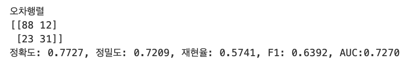

예측 정확도가 77.27%, 재현율은 57.41%로 측정되었다. 하지만 전체 데이터의 65.1%가 Negative이므로 재현율 성능에 조금 더 초점을 맞추도록 하자.
먼저 정밀도 재현율 곡선을 보고 임곗값별 정밀도와 재현율 값의 변화를 확인해보자.

pred_proba_c1 = lr_clf.predict_proba(X_test)[:, 1]
precision_recall_curve_plot(y_test, pred_proba_c1)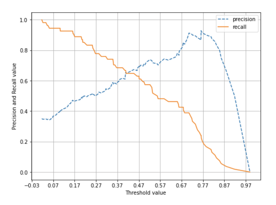

재현율 곡선을 보면 임곗값 0.42 정도에서 정밀도와 재현율이 같아지는 것을 볼 수 있다. 하지만 두 지표 다 0.7도 안된다.

3. 최솟값을 평균값으로 대체

임곗값 조작 전에 데이터 값을 점검해보자.

diabetes_data.describe()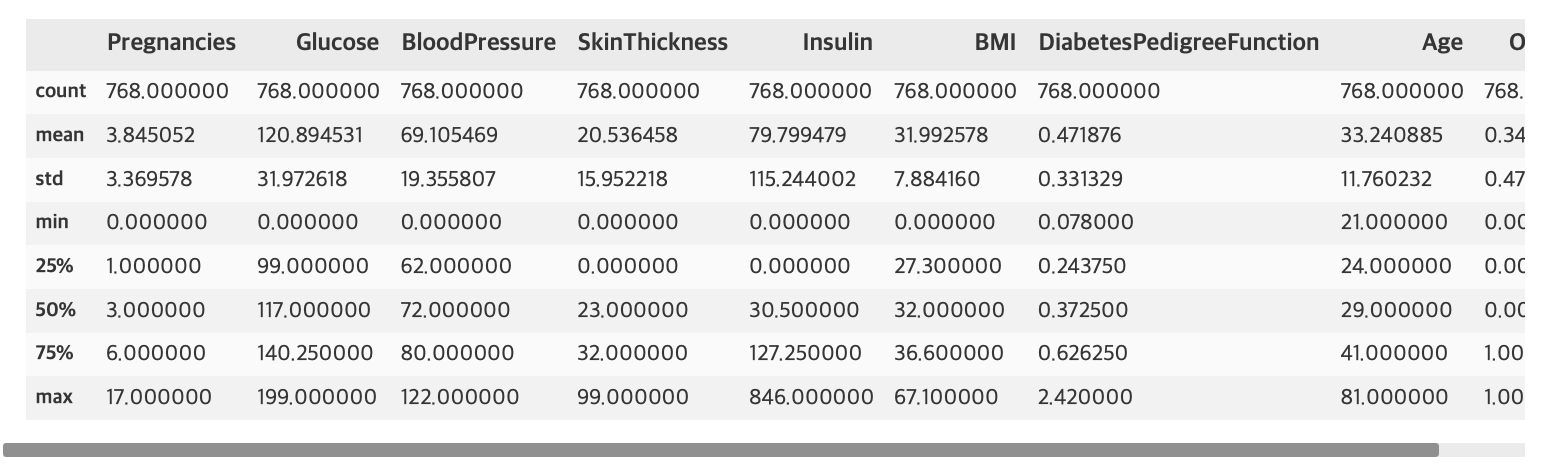

다른것보다 min() 값이 0인 것이 많이 눈에 띈다. 특히 Glucose는 포도당 수치인데 이것이 0인 것은 말이 안된다. Glucose의 히스토그램을 살펴보자.

plt.hist(diabetes_data['Glucose'], bins=10)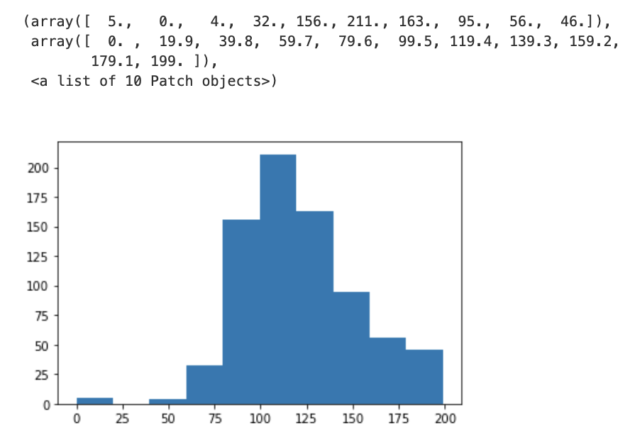

min()이 0으로 되어있는 피처에 대해 몇 퍼센트가 0인지 확인해보자. 여기서 확인할 피처는 Glucose, BloodPressure, SkinThickness, Insulin, BMI이다.

zero_features = ['Glucose', 'BloodPressure', 'SkinThickness', 'Insulin', 'BMI']
total_count = diabetes_data['Glucose'].count()
for feature in zero_features:
    zero_count = diabetes_data[diabetes_data[feature]==0][feature].count()
    print('{0} 0 건수는 {1}, 퍼센트는 {2:.2f} %'.format(feature, zero_count, 100*zero_count/total_count))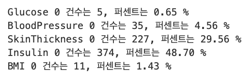

SkinThickness와 Insulin의 0 값이 각각 29.59%, 48.70%로 꽤나 많다. 하지만 데이터 갯수가 많은 것이 아니기에 위 피처의 0 값을 삭제하기보다 평균값으로 대체하자.

mean_zero_features = diabetes_data[zero_features].mean()
diabetes_data[zero_features] = diabetes_data[zero_features].replace(0, mean_zero_features)

4. 피처 스케일링

0 값을 평균값으로 대체한 데이터 세트에 피처 스케일링을 적용해 변환해보자. 일반적으로 로지스틱 회귀의 경우 숫자 데이터에 스케일링을 적용하는 것이 좋다.

X = diabetes_data.iloc[:, :-1]
y = diabetes_data.iloc[:, -1]

# StandardScaler 클래스를 이용해 피처 데이터 세트에 일괄적으로 스케일링 적용
scaler = StandardScaler()
X_scaled = scaler.fit_transform(X)

X_train, X_test, y_train, y_test = train_test_split(X, y, test_size=0.2, random_state=156, stratify=y)

lr_clf = LogisticRegression()
lr_clf.fit(X_train, y_train)
pred = lr_clf.predict(X_test)
pred_proba = lr_clf.predict_proba(X_test)[:, 1]

get_clf_eval(y_test, pred, pred_proba)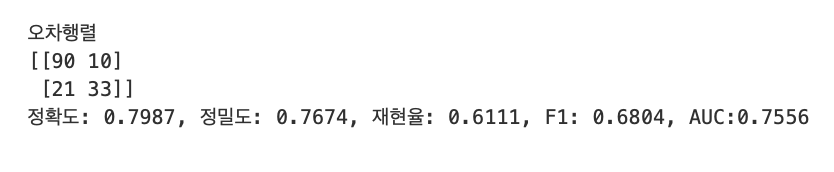

데이터 변환과 스케일링을 통해 정확도, 정밀도, 재현율, F1의 값이 각각 0.7727, 0.7209, 0.5741, 0.6392 에서 0.7987, 0.7674, 0.6111, 0.6804 로 개선되었다. 하지만 여전히 재현율의 수치는 개선이 필요해 보이므로 임곗값을 변화시키면서 확인해보자.

thresholds = [0.3, 0.33, 0.36, 0.39, 0.42, 0.45, 0.48, 0.50]
pred_proba = lr_clf.predict_proba(X_test)
get_eval_by_threshold(y_test, pred_proba[:, 1].reshape(-1, 1), thresholds)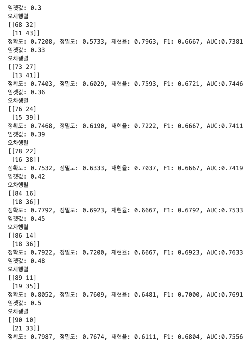

정확도와 정밀도를 희생하고 재현율을 높이는데 가장 좋은 임곗값은 0.30 으로 재현율이 0.7963 이다. 하지만 정밀도가 0.5733으로 매우 저조하니 극단적인 선택으로 보인다. 전체적인 성능 평가 지표를 유지하면서 재현율을 악간 상승시키는 임곗값 0.48 이 좋은 임곗값으로 보이고, 이때 정확도: 0.8052, 정밀도: 0.7609, 재현율: 0.6481, F1: 0.7000, ROC AUC:0.7691 이다.

5. 임곗값 수정 및 최종 예측

임곗값을 0.48로 낮춘 상태로 다시 예측을 해보자. 단, 사이킷런의 predict() 메서드는 임곗값을 마음대로 바꿀 수 없으므로 별도의 로직으로 구해야한다.

binarizer = Binarizer(threshold=0.48)

# 위에서 구한 lr_clf의 predict_proba() 예측 확률 array에서 1에 해당하는 칼럼값을 Binarizer 변환
pred_th_048 = binarizer.fit_transform(pred_proba[:, 1].reshape(-1, 1))

get_clf_eval(y_test, pred_th_048, pred_proba[:, 1])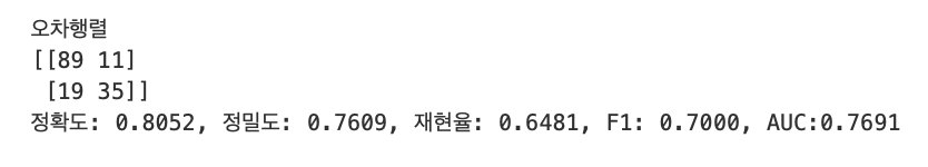

Source: 파이썬 머신러닝 완벽 가이드 / 위키북스