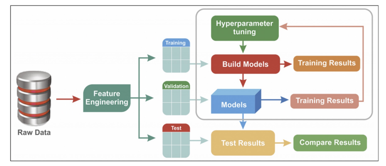
하이퍼파마리터 튜닝은 모델의 성능을 확보하기 위해 조절하는 설정 값 을 의미한다.

예를 들면 Decision Tree에서는 max_depth 가 있다.
물론 반복문을 사용할 수 있지만, 더 쉬운 방법이 있다!

이번에도 와인 데이터를 분류하는 모델을 만들고, 다양한 max_depth 값을 입력해보자

　

1. 데이터 불러오기

데이터

import pandas as pd

red_wine = pd.read_csv(red_url, sep=';')
white_wine = pd.read_csv(white_url, sep=';')

red_wine['color'] = 1
white_wine['color'] = 0

wine = pd.concat([red_wine, white_wine])

wine['taste'] = [1. if grade>5 else 0. for grade in wine['quality']]

X = wine.drop(['taste', 'quality'], axis=1)
y = wine['taste']

이번에도 두 데이터를 불러와서 color 컬럼을 만든 뒤, 하나로 합쳐줬다.

　

2. GridSearch CV

• cv : cross validation
• 수정하고 싶은 파라미터를 dic 으로 정의하면 된다.

(1) 모델 만들기

from sklearn.model_selection import GridSearchCV
from sklearn.tree import DecisionTreeClassifier

모델은 지금까지 사용했던 Decision Tree를 사용한다.

　

params = {'max_depth' : [2, 4, 7, 10]}
wine_tree = DecisionTreeClassifier(max_depth=2, random_state=13)

gs = GridSearchCV(estimator=wine_tree, param_grid=params, cv=5)
gs.fit(X, y)

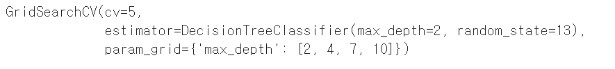
GridSearchCV(estimator=wine_tree, param_grid=params, cv=5)
estimator : 사용하는 모델
param_grid : 수정하는 파라미터
cv : kfold에서 n_splits

fit 시킬 때, tain-test split을 하지 않아도 GridSearchCV가 자동으로 나눠서 해준다.
이제 GridSearchCV가 kfold를 5회 하고, max_depth는 2, 4, 7, 10 으로 바꿔가면서 모델 학습을 한다.

　

(2) 성능 확인

import pprint

pp = pprint.PrettyPrinter(indent=4)
pp.pprint(gs.cv_results_)

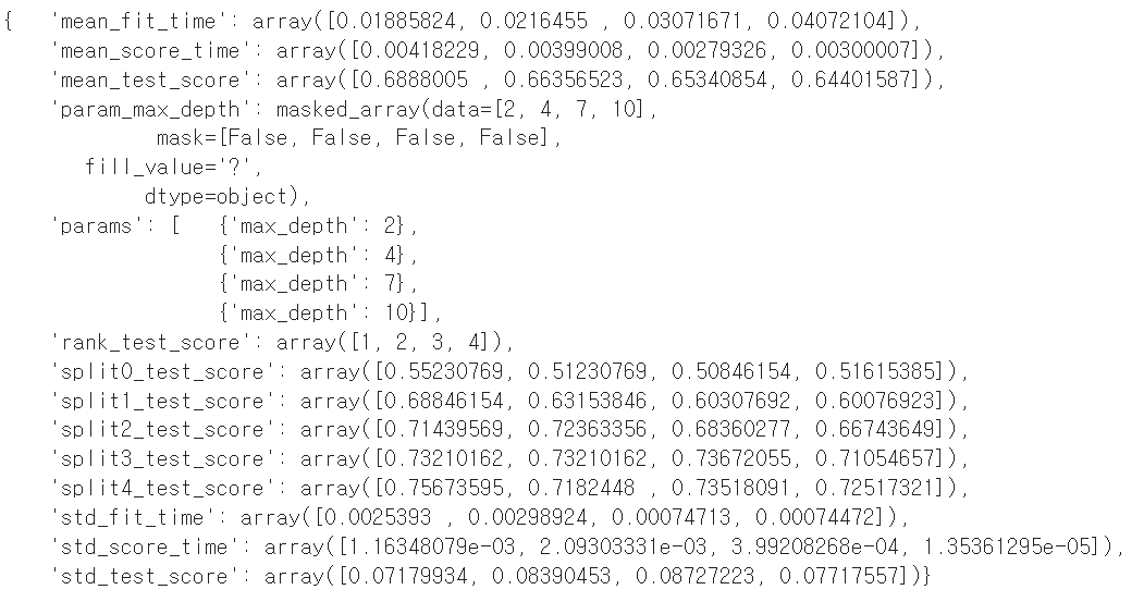
cv_results_ 를 이용하면 입력한 max_depth 들의 acc들을 한번에 볼 수 있다.
'rank_test_score': array([1, 2, 3, 4]) : 2, 4, 7, 10 순서대로 1, 2, 3, 4 등

　

가장 좋은 결과만 보고싶다면
best_estimator_, best_score_, best_params_, best_index_ 를 출력하면 된다.

print("gs.best_estimator_ : ", gs.best_estimator_)
print("gs.best_score_     : ", gs.best_score_)
print("gs.best_params_    : ", gs.best_params_)
print("gs.best_index_     : ", gs.best_index_)

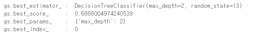
내가 입력한 값 중, 2일때가 가장 최적의 결과를 반환하고 그때 acc는 약69% 이다.

　

3. Pipeline에 적용

from sklearn.pipeline import Pipeline
from sklearn.tree import DecisionTreeClassifier
from sklearn.preprocessing import StandardScaler

estimators = [('scaler', StandardScaler()),
             ('clf', DecisionTreeClassifier(random_state=13))]

pipe = Pipeline(estimators)

먼저 StandardScaler와 DecisionTreeClassifier 로 이뤄진 파이프라인을 구축한다.

　

이제 GridSearchCV를 이용해 파이프라인 안에 있는 DecisionTree의 max_depth 값을 변경해보자!
파이프라인에서 특정 단계의 파라미터를 호출할때는 언더바 2개! 잊지말자!!

param_pipe = [{'clf__max_depth' : [2, 4, 7, 10]}]   

gs_p = GridSearchCV(estimator=pipe, param_grid=param_pipe, cv=5)
gs_p.fit(X,y)

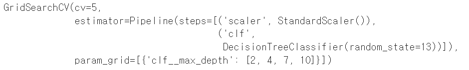
GridSearchCV 에 입력하는 것은 위와 동일하다.

　

이번에도 결과를 출력해보자.

pp = pprint.PrettyPrinter(indent=4)
pp.pprint(gs_p.cv_results_)

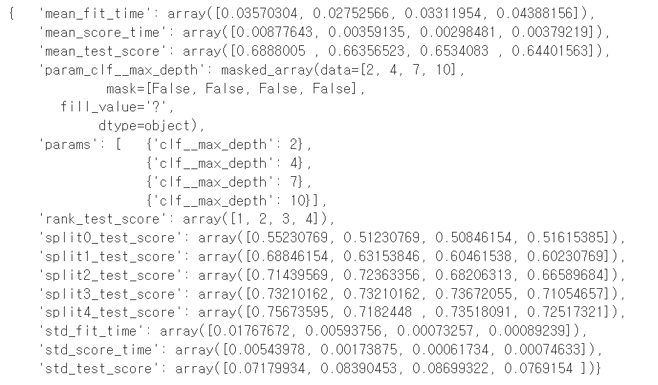
이번에도 1, 2, 3, 4 순으로 좋은 값이라는 결과가 나왔당!

　

print("gs_p.best_estimator_ : ", gs_p.best_estimator_)
print("gs_p.best_score_     : ", gs_p.best_score_)
print("gs_p.best_params_    : ", gs_p.best_params_)
print("gs_p.best_index_     : ", gs_p.best_index_)

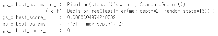
acc 값도 큰 차이가 없다.

　

4. 결과 정리

위에 정신없이 적혀진 결과들을 한눈에 보기 쉽게 표로 정리해보쟈

score_df = pd.DataFrame(gs_p.cv_results_)
score_df[['params', 'rank_test_score', 'mean_test_score', 'std_test_score']]

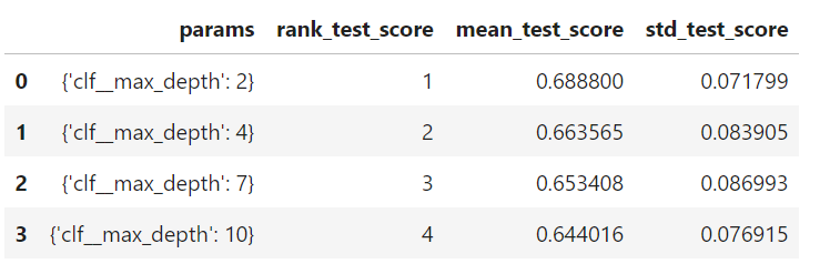
그중 내가 필요한 ['params', 'rank_test_score', 'mean_test_score', 'std_test_score'] 만 따로 출력해봤다!