Adaptive KNN (AdaKNN) Classifier

Introduction

The Adaptive k-Nearest Neighbors (k-NN) Classifier is an extension of the traditional k-NN algorithm, which is widely used for classification and regression tasks in machine learning. Unlike the standard k-NN that uses a fixed number of nearest neighbors for all predictions, the Adaptive k-NN algorithm adjusts the number of neighbors (k) based on the local density of points, aiming to improve classification accuracy, especially in areas where data points are not uniformly distributed.

Background and Theory

The k-NN algorithm operates on a simple principle: it classifies a new sample based on the majority vote of its k nearest neighbors in the feature space. The standard k-NN algorithm uses a fixed k value, which can be suboptimal in varying density regions. The Adaptive k-NN Classifier, however, dynamically adjusts k for each query point, taking into consideration the local density of neighbors. This adjustment allows for more flexible decision boundaries and can lead to improved performance in heterogeneous datasets.

How the Algorithm Works

Steps

1. Calculate Distance: Compute the distance between the query point and all points in the training dataset.
2. Determine Local Density: Estimate the density around the query point. This can be done using methods like the distance to the $n$ th nearest neighbor or the average distance to the nearest $n$ neighbors.
3. Adjust $k$ Value: Adjust the value of $k$ based on the local density. For denser areas, a higher $k$ might be used, while sparser areas might use a lower $k$.
4. Classify: Identify the $k$ nearest neighbors to the query point based on the adjusted $k$ value. Classify the query point based on the majority vote among these neighbors.

Local Density Calculation

Let $X = \{x_1, x_2, \cdots, x_n\}$ be the set of training samples and $x$ be the query point. The local density $\rho$ at $x$ is estimated by:

where:

• $d(x, x_{(i)})$ denotes the distance between the query point $x$ and its $i$ th nearest neighbor $x_{(i)}$ in the training set.
• $N$ is a predefined parameter indicating the number of nearest neighbors considered for estimating the local density.

Adaptive k Value Determination

The adaptive number of neighbors $k_{a}$, to be considered for classifying $x$ is defined as:

where:

• $k_{b}$ is a predetermined base number of neighbors.
• $g(\rho(x))$ is a scaling function that adjusts $k_{b}$ based on the estimated local density $\rho(x)$.

Classification Decision

The classification of the query point $x$ is determined by the majority vote among its $k_a$ nearest neighbors:

where $\text{Class}(x_{(i)})$ denotes the class label of the $i$ th nearest neighbor of $x$.

Implementation

Parameters

• n_density: int, default = 10
  Number of nearest neighbors to estimate the local density
  
• min_neighbors : int, default = 5
  Minimum number of neighbors to be considered for averaging
  
• max_neighbors: int, default = 20
  Maximum number of neighbors to be considered
  

Examples

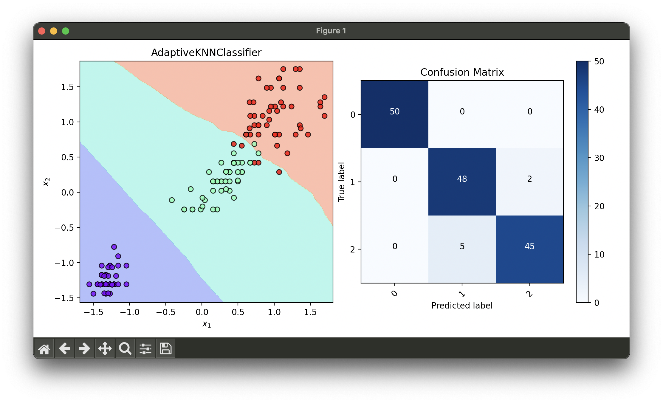
Test with iris flower dataset and reduce dimensionality via SFS using GaussianNaiveBayes as a base estimator:

from luma.classifier.naive_bayes import GaussianNaiveBayes
from luma.classifier.neighbors import AdaptiveKNNClassifier
from luma.preprocessing.scaler import StandardScaler
from luma.reduction.selection import SFS
from luma.model_selection.split import TrainTestSplit
from luma.model_selection.search import GridSearchCV
from luma.visual.evaluation import DecisionRegion, ConfusionMatrix

from sklearn.datasets import load_iris
import matplotlib.pyplot as plt
import numpy as np


X, y = load_iris(return_X_y=True)

X_train, X_test, y_train, y_test = TrainTestSplit(X, y,
                                                  test_size=0.2,
                                                  random_state=42).get

sc = StandardScaler()
X_train_std = sc.fit_transform(X_train)
X_test_std = sc.fit_transform(X_test)

sfs = SFS(estimator=GaussianNaiveBayes(),
          n_features=2,
          test_size=0.2,
          cv=5,
          random_state=42,
          verbose=True)

sfs.fit(X_train_std, y_train)
X_train_sfs = sfs.transform(X_train_std)
X_test_sfs = sfs.transform(X_test_std)

param_grid = {'n_density': range(2, 20)}

grid = GridSearchCV(estimator=AdaptiveKNNClassifier(),
                    param_grid=param_grid,
                    cv=5,
                    refit=True,
                    random_state=42)

grid.fit(X_train_sfs, y_train)
knn_best = grid.best_model

X_concat = np.concatenate((X_train_sfs, X_test_sfs))
y_concat = np.concatenate((y_train, y_test))

fig = plt.figure(figsize=(10, 5))
ax1 = fig.add_subplot(1, 2, 1)
ax2 = fig.add_subplot(1, 2, 2)

dec = DecisionRegion(knn_best, X_concat, y_concat)
dec.plot(ax=ax1)

conf = ConfusionMatrix(y_concat, knn_best.predict(X_concat))
conf.plot(ax=ax2, show=True)

# Best params: {'n_density': 5}
# Best score: 0.9583333333333334

Applications and Use Cases

The Adaptive k-NN Classifier is particularly useful in scenarios where data points are unevenly distributed across the feature space, such as:

• Image recognition, where the density of features can vary significantly across different parts of an image.
• Fraud detection in financial transactions, where fraudulent activities may cluster in certain areas but not others.
• Medical diagnosis, where patient data might cluster differently based on conditions or demographics.

Strengths and Limitations

• Strengths
  • Improved accuracy in heterogeneous density regions by adapting to local data distribution.
  • Flexibility in handling various types of data without the need for uniform scaling.
  • Intuitive understanding and implementation, similar to the standard k-NN algorithm.
• Limitations
  • Increased computational complexity due to the need for calculating local densities and adjusting $k$.
  • Selection of the density estimation method and base $k$ value can significantly influence performance.
  • Potentially more sensitive to noise, especially in sparse regions.

Advanced Topics and Further Reading

For those interested in exploring beyond the basics of the Adaptive k-NN Classifier, the following topics are recommended:

• Weighted k-NN: Incorporating weights based on the distance or other relevance metrics to improve classification accuracy.
• Locality-Sensitive Hashing (LSH): Techniques for reducing the dimensionality and speeding up neighbor search in high-dimensional spaces.
• Cross-validation for Hyperparameter Tuning: Methods for selecting optimal base $k$ values and other parameters through systematic evaluation.

References

1. Cover, T., and Hart, P. "Nearest neighbor pattern classification." IEEE transactions on information theory 13.1 (1967): 21-27.
2. Hastie, T., Tibshirani, R., and Friedman, J. "The Elements of Statistical Learning." Springer Series in Statistics (2009).
3. Samworth, R. "Optimal weighted nearest neighbour classifiers." Annals of Statistics 39.5 (2011): 2733-2763.