Weighted KNN Classifier

Introduction

The Weighted K-Nearest Neighbors (KNN) Classifier enhances the conventional KNN algorithm by introducing a weighting scheme for the neighbors based on their distance from the query point. This method not only considers the nearest neighbors but also quantifies their relevance, making the algorithm more sensitive and adaptable to the local data structure. It's particularly beneficial in scenarios where data points are not uniformly distributed.

Background and Theory

KNN belongs to the family of instance-based, lazy learning algorithms. It operates on the premise that similar instances have similar outcomes. Traditional KNN classifies an instance based on the majority vote of its nearest neighbors. The weighted KNN variant takes this a step further by attributing a weight to each neighbor according to their distance, thus prioritizing nearer neighbors over the farther ones. This approach can significantly enhance performance in heterogeneous data distributions.

How the Algorithm Works

Steps

1. Initialization: Choose the number $k$ of neighbors and decide on a distance metric (e.g., Euclidean, Manhattan).
2. Distance Calculation: Compute the distance between the query instance and every instance in the training set.
3. Neighbor Identification: Sort the distances and identify the top $k$ nearest neighbors.
4. Weight Assignment: Assign weights to these $k$ neighbors. The weight can be inversely proportional to the distance, ensuring that closer neighbors have a greater influence on the final prediction.
5. Result Aggregation:
   • For classification, compute the weighted sum of votes for each class and predict the class with the maximum weighted vote.
   • For regression, calculate the weighted average of the neighbors' values.

Mathematical Formulation

Let $x$ denote the query point and $x_i$ represent a neighbor within the training set. The distance between $x$ and $x_i$ is denoted as $d(x, x_i)$. A common weighting function is $w_i = {1}/{d(x, x_i)^2}$, emphasizing closer neighbors more significantly.

For classification, the prediction is given by:

where $y_i$ is the class label of the $i$-th neighbor, and $\mathbf{1}(y_i = j)$ is an indicator function.

Implementation

Parameters

• n_neighbors: int, default = 5 Number of neighbors to be considered close
  

Examples

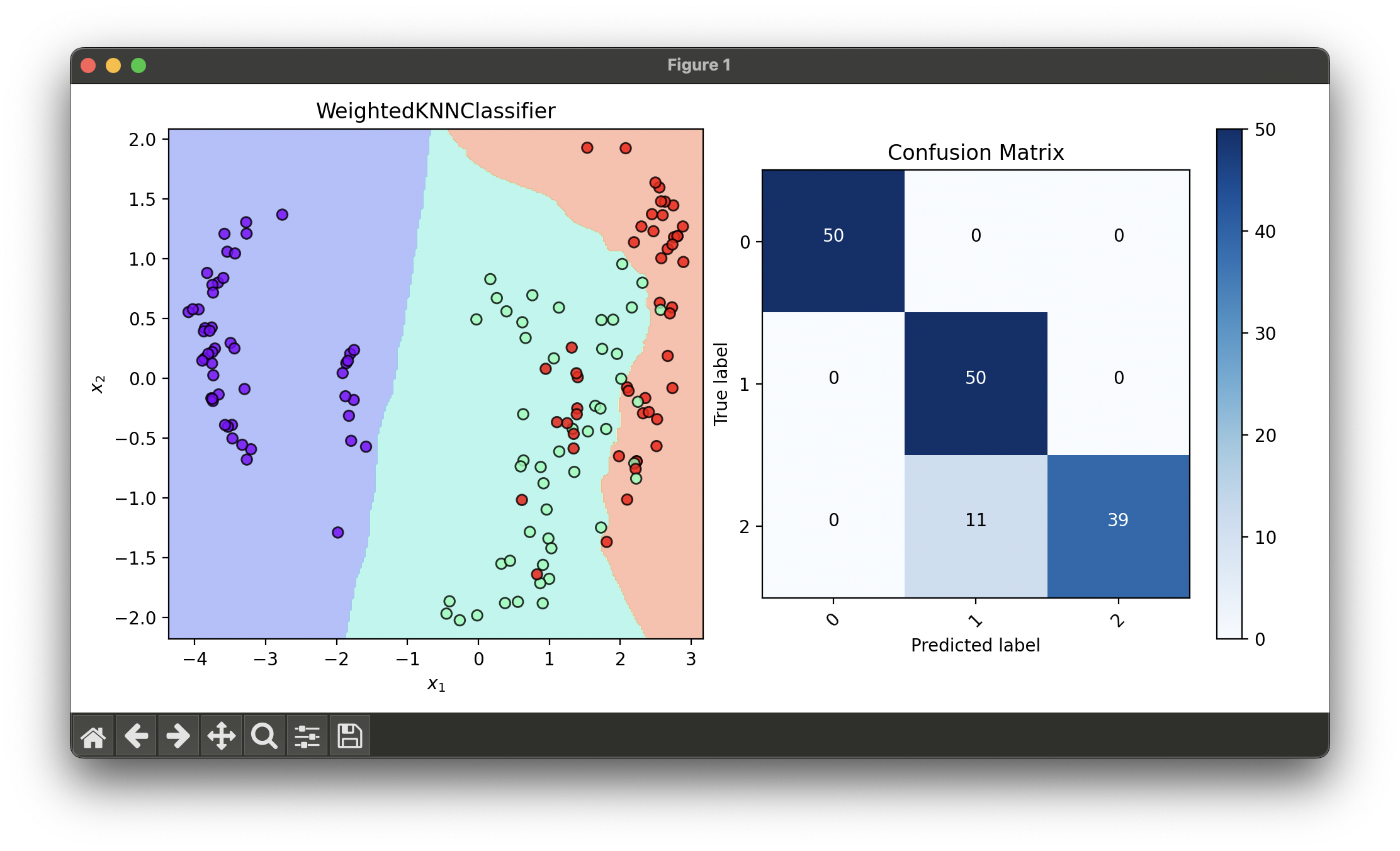
Test with iris flower dataset and reduce dimensionality via KernelPCA:

from luma.classifier.neighbors import WeightedKNNClassifier
from luma.preprocessing.scaler import StandardScaler
from luma.reduction.linear import KernelPCA
from luma.model_selection.split import TrainTestSplit
from luma.model_selection.search import GridSearchCV
from luma.visual.evaluation import DecisionRegion, ConfusionMatrix

from sklearn.datasets import load_iris
import matplotlib.pyplot as plt
import numpy as np

X, y = load_iris(return_X_y=True)

X_train, X_test, y_train, y_test = TrainTestSplit(X, y,
                                                  test_size=0.2,
                                                  random_state=42).get

sc = StandardScaler()
X_train_std = sc.fit_transform(X_train)
X_test_std = sc.fit_transform(X_test)

kpca = KernelPCA(n_components=2, gamma=0.1, kernel='rbf')
X_train_tr = kpca.fit_transform(X_train_std)
X_test_tr = kpca.fit_transform(X_test_std)

param_grid = {'n_neighbors': range(2, 20)}

grid = GridSearchCV(estimator=WeightedKNNClassifier(),
                    param_grid=param_grid,
                    cv=5,
                    refit=True,
                    random_state=42)

grid.fit(X_train_tr, y_train)
wknn_best = grid.best_model

X_concat = np.concatenate((X_train_tr, X_test_tr))
y_concat = np.concatenate((y_train, y_test))

fig = plt.figure(figsize=(10, 5))
ax1 = fig.add_subplot(1, 2, 1)
ax2 = fig.add_subplot(1, 2, 2)

dec = DecisionRegion(wknn_best, X_concat, y_concat)
dec.plot(ax=ax1)

conf = ConfusionMatrix(y_concat, wknn_best.predict(X_concat))
conf.plot(ax=ax2, show=True)

# Best params: 'n_neighbors': 12
# Best score: 0.925

Applications and Use Cases

• Medical Diagnosis: Enhancing the accuracy of diagnosing diseases by considering the proximity of symptoms and test results to known cases.
• Financial Fraud Detection: Identifying and prioritizing suspicious transactions based on similarities to previously confirmed fraudulent activities.
• Recommendation Systems: Improving recommendations by weighting user preferences and behaviors according to similarity and proximity metrics.
• Real Estate Pricing: Estimating property values by weighing the prices of nearby properties, with closer properties having more influence.

Strengths and Limitations

• Strengths
  • Improved accuracy over standard KNN by considering the relative importance of neighbors.
  • Flexible to the choice of distance metric and weighting function, allowing customization for specific applications.
  • Effective in handling non-linear data distributions due to its instance-based nature.
• Limitations
  • Increased computational cost due to distance calculation and sorting, especially in large datasets.
  • Sensitivity to the choice of $k$, distance metric, and weighting function, which can significantly impact performance.
  • Prone to biases from imbalanced data sets unless carefully weighted or sampled.

Advanced Topics and Further Reading

• Dynamic Weighting Schemes: Exploring adaptive weighting methods that adjust based on local data characteristics or through optimization techniques.
• Dimensionality Reduction: Techniques such as PCA (Principal Component Analysis) to reduce the feature space, improving efficiency and potentially accuracy.
• Ensemble Methods: Combining weighted KNN with other algorithms to form robust predictive models.
• Optimizing $k$ and Distance Metrics: Advanced strategies for selecting the optimal $k$ and the most appropriate distance metric through cross-validation and domain-specific insights.

References

1. Dudani, S. A. (1976). The distance-weighted k-nearest-neighbor rule. IEEE Transactions on Systems, Man, and Cybernetics, SMC-6(4), 325-327.
2. Hechenbichler, K., & Schliep, K. (2004). Weighted k-nearest-neighbor techniques and ordinal classification. Discussion Paper 399, SFB 386, Ludwig-Maximilians University Munich.
3. Altman, N. S. (1992). An introduction to kernel and nearest-neighbor nonparametric regression. The American Statistician, 46(3), 175-185.
4. Hastie, T., Tibshirani, R., & Friedman, J. (2009). The Elements of Statistical Learning: Data Mining, Inference, and Prediction. Springer Series in Statistics, Springer.
5. James, G., Witten, D., Hastie, T., & Tibshirani, R. (2013). An Introduction to Statistical Learning with Applications in R. Springer Texts in Statistics, Springer.