K-Nearest Neighbors (KNN) Classifier

Introduction

The K-Nearest Neighbors (KNN) classifier is a type of instance-based learning, or lazy learning, where the function is only approximated locally, and all computation is deferred until function evaluation. It is one of the simplest of all machine learning algorithms, primarily used for classification, and operates on the principle that similar things exist in close proximity.

Background and Theory

In KNN, the classification of an observation is determined by a plurality vote of its neighbors, with the observation being assigned to the class most common among its $k$ nearest neighbors measured by a distance metric (e.g., Euclidean distance). $k$ is a positive integer, typically small. If $k = 1$, then the object is simply assigned to the class of its nearest neighbor.

Distance Metrics

The choice of distance metrics can significantly influence the performance of KNN. Common distance metrics include:

• Euclidean Distance: The most common choice, defined for two points $x$ and $y$ in an $n$-dimensional space as
  $d(x, y) = \sqrt{\sum_{i=1}^{n} (x_i - y_i)^2}$
  
• Manhattan Distance: Used in taxicab geometry, computed as
  $d(x, y) = \sum_{i=1}^{n} |x_i - y_i|$
  
• Minkowski Distance: A generalization of both Euclidean and Manhattan distances, defined as
  $d(x, y) = \left(\sum_{i=1}^{n} |x_i - y_i|^p\right)^{1/p}$
  

How the Algorithm Works

Steps

1. Choose the number of $k$: Determine the value of $k$, the number of nearest neighbors to consider. It can be selected based on cross-validation.
2. Select a distance metric: Choose a method to measure the distance between different instances.
3. Find the $k$ nearest neighbors of the new data point: Calculate the distance between the new point and all points in the training set, selecting the $k$ smallest distances corresponding to the $k$ nearest neighbors.
4. Vote for labels: The new data point is assigned to the class most common among its $k$ nearest neighbors.
5. Handle ties (if necessary): Implement a tie-breaking rule if the vote among the nearest neighbors results in a tie.

Mathematical Formulation

Given a dataset $\mathcal{D}$ containing $n$ samples with their corresponding labels, the task is to classify a new sample $x$. The distance between $x$ and each sample in $\mathcal{D}$ is calculated using a chosen distance metric. The $k$ samples in $\mathcal{D}$ with the smallest distance to $x$ are identified, and the frequency of each class within these $k$ samples is counted:

The predicted class $y$ for $x$ is then given by:

Implementation

Parameters

• n_neighbors: int, default = 5
  Number of neighbors to be considered close
  

Examples

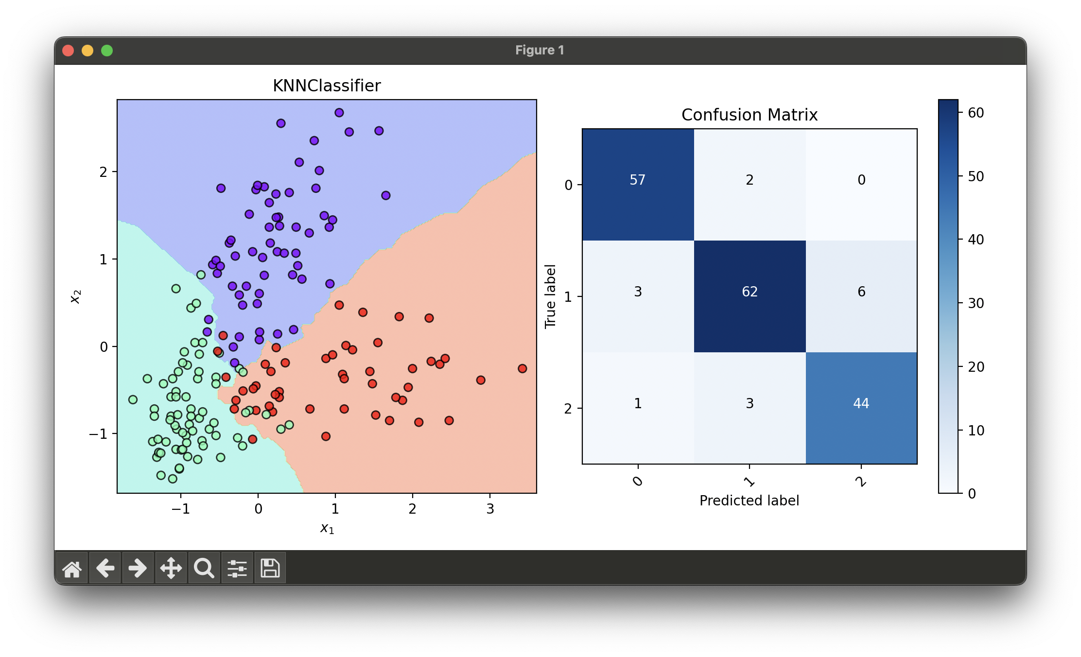
Test with wine dataset and reduce dimensionality with RFE using GaussianNaiveBayes as base estimator:

from luma.classifier.naive_bayes import GaussianNaiveBayes
from luma.classifier.neighbors import KNNClassifier
from luma.preprocessing.scaler import StandardScaler
from luma.reduction.selection import RFE
from luma.model_selection.split import TrainTestSplit
from luma.model_selection.search import GridSearchCV
from luma.visual.evaluation import DecisionRegion, ConfusionMatrix

from sklearn.datasets import load_wine
import matplotlib.pyplot as plt
import numpy as np


X, y = load_wine(return_X_y=True)

X_train, X_test, y_train, y_test = TrainTestSplit(X, y,
                                                  test_size=0.2,
                                                  random_state=42).get

sc = StandardScaler()
X_train_std = sc.fit_transform(X_train)
X_test_std = sc.fit_transform(X_test)

rfe = RFE(estimator=GaussianNaiveBayes(),
          n_features=2,
          step_size=1, 
          cv=5,
          random_state=42,
          verbose=True)

rfe.fit(X_train_std, y_train)
X_train_rfe = rfe.transform(X_train_std)
X_test_rfe = rfe.transform(X_test_std)

param_grid = {'n_neighbors': range(2, 10)}

grid = GridSearchCV(estimator=KNNClassifier(),
                    param_grid=param_grid,
                    cv=5,
                    refit=True,
                    random_state=42)

grid.fit(X_train_rfe, y_train)
knn_best = grid.best_model

X_concat = np.concatenate((X_train_rfe, X_test_rfe))
y_concat = np.concatenate((y_train, y_test))

fig = plt.figure(figsize=(10, 5))
ax1 = fig.add_subplot(1, 2, 1)
ax2 = fig.add_subplot(1, 2, 2)

dec = DecisionRegion(knn_best, X_concat, y_concat)
dec.plot(ax=ax1)

conf = ConfusionMatrix(y_concat, knn_best.predict(X_concat))
conf.plot(ax=ax2, show=True)

# RFE best score: 0.94408766
# RFE final features: (9, 12)
# Best params: {'n_neighbors': 5}
# Best score: 0.9299539170506913

Applications and Use Cases

KNN is widely used in a variety of applications, such as:

• Image Recognition: Identifying objects or people within an image.
• Recommendation Systems: Suggesting products or media similar to what a user likes.
• Medical Diagnosis: Classifying patient cases based on similarity to previous cases.

Strengths and Limitations

• Strengths
  • Simple to understand and implement.
  • Naturally handles multi-class cases.
  • Learning time is negligible since it involves no explicit model training.
• Limitations
  • High prediction time for large datasets.
  • Performance depends heavily on the choice of (k) and the distance metric.
  • Sensitive to irrelevant or redundant features since all features contribute equally to the distance computation.

Advanced Topics and Further Readings

• Feature Weighting: Techniques to assign different weights to features based on their importance.
• Dimensionality Reduction: Methods like PCA (Principal Component Analysis) to reduce the number of variables under consideration to improve the performance of KNN.
• Efficient Search Algorithms: Implementing tree-based data structures like KD-trees or ball trees to speed up the search for nearest neighbors.

References

1. Cover, Thomas, and Peter Hart. "Nearest neighbor pattern classification." IEEE transactions on information theory 13.1 (1967): 21-27.
2. Dasarathy, Belur V., ed. "Nearest neighbor (NN) norms: NN pattern classification techniques." IEEE Computer Society Press, 1991.
3. Friedman, Jerome, Trevor Hastie, and Robert Tibshirani. "The elements of statistical learning." Vol. 1. No. 10. New York: Springer series in statistics, 2001.