Bernoulli Naive Bayes

Introduction

Bernoulli Naive Bayes is a variant of the Naive Bayes algorithm, designed specifically for binary/boolean features. It operates on the principle that features are independent given the class, but unlike its counterparts, it assumes that all features are binary-valued (Bernoulli distributed). This model is particularly effective in text classification problems where the presence or absence of a feature (e.g., a word) is more significant than its frequency.

Background and Theory

Naive Bayes classifiers apply Bayes' theorem with the assumption of independence among predictors. Bernoulli Naive Bayes is tailored for dichotomous variables and models the presence or absence of a characteristic with a Bernoulli distribution. This approach is suited for datasets where features can be encoded as binary variables, representing the presence or absence of a feature.

Bayes' Theorem

The foundation of Naive Bayes classification is Bayes' Theorem, which describes the probability of an event, based on prior knowledge of conditions that might be related to the event. It is mathematically expressed as:

where:

• $P(A|B)$ is the posterior probability of class $A$ given predictor $B$.
• $P(B|A)$ is the likelihood of predictor $B$ given class $A$.
• $P(A)$ is the prior probability of class $A$.
• $P(B)$ is the prior probability of predictor $B$.

Naive Bayes Classifier

The Naive Bayes classifier simplifies to computing the posterior probability of each class given a set of predictors and assuming that the predictors are independent of each other given the class. For a set of predictors $X_1, X_2,\cdots, X_n$ and a class $C$, the posterior probability is:

Bernoulli Distribution

The Bernoulli distribution is a discrete distribution having two possible outcomes: 1 (success) with probability $p$, and 0 (failure) with probability $1-p$. For a random variable $X$ following a Bernoulli distribution, the probability mass function (PMF) is given by:

where $x \in \{0, 1\}$.

Maximum Likelihood Estimation (MLE)

In Bernoulli Naive Bayes, we are interested in estimating the probability $p_{j|y}$ that a feature $j$ is present (i.e., equals 1) in a given class $y$. The likelihood of observing a dataset given the parameters can be formulated as the product of the probabilities of observing each individual data point. The goal of MLE in this context is to find the probability $p_{j|y}$ that maximizes this likelihood.

Given a dataset, the MLE for the probability $p_{j|y}$ is calculated as the ratio of:

• The number of times feature $j$ appears in samples of class $y$, to
• The total number of samples of class $y$.

Mathematically, this is expressed as:

where:

• $I(\cdot)$ is an indicator function that is 1 if the condition is true and 0 otherwise,
• $n$ is the total number of samples,
• $y_i$ is the class of the $i$ th sample,
• $x_{ij}$ is the $j$ th feature of the $i$ th sample.

Smoothing

To deal with the issue of zero probabilities (for instance, when a feature does not appear in any sample of a class in the training set), Laplace smoothing (or add-one smoothing) is often applied:

where $\alpha$ is the smoothing parameter, typically set to 1. This adjustment ensures that each class-feature combination has a non-zero probability.

How the Algorithm Works

Steps

1. Data Preparation: Convert all features into binary (0 or 1) values indicating the absence or presence of a feature.
2. Parameter Estimation: Calculate the probabilities of feature presence (and absence) for each class in the training dataset.
3. Posterior Probability Calculation: Use these probabilities along with the prior probability of each class to calculate the posterior probabilities of the classes given an observation.
4. Decision Making: Assign the class with the highest posterior probability to the new observation.

Mathematical Formulation

For a binary feature $x_i$ and class $c_j$, the probability of observing $x_i$ given $c_j$ is modeled as:

where $p_{ij}$ is the probability of feature $i$ being present (1) in class $j$, estimated from the training data.

The posterior probability for class $c_j$ given an observation $\mathbf{x} = (x_1, \cdots, x_n)$ is calculated using Bayes' theorem:

Classification is performed by selecting the class $c_j$ that maximizes $P(c_j | \mathbf{x})$.

Implementation

Parameters

No parameters.

Examples

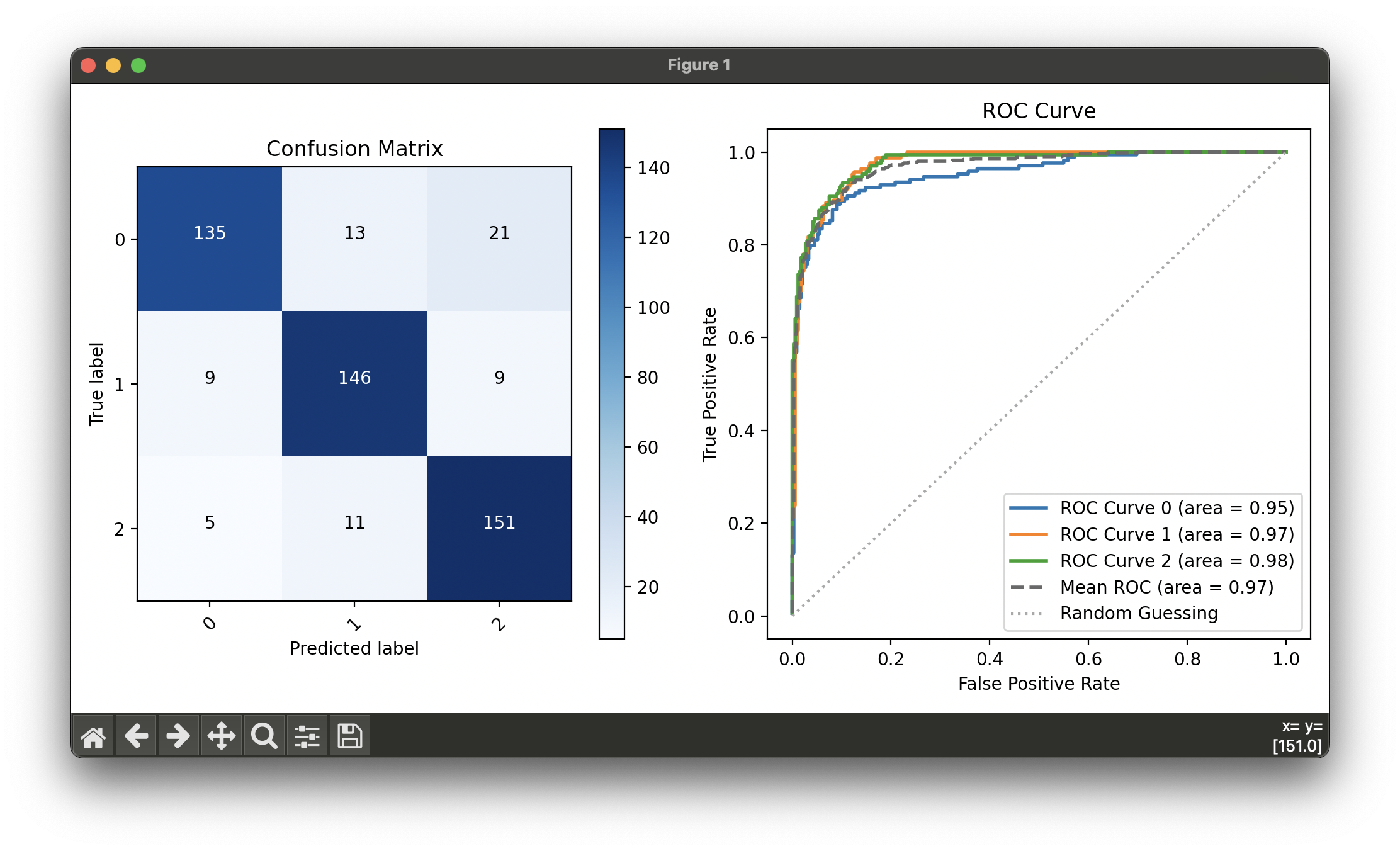
Test with synthesized binary classification dataset with 3 classes:

from luma.classifier.naive_bayes import BernoulliNaiveBayes
from luma.model_selection.split import TrainTestSplit
from luma.visual.evaluation import ConfusionMatrix, ROCCurve

from sklearn.datasets import make_classification
import matplotlib.pyplot as plt
import numpy as np


X, y = make_classification(n_samples=500, 
                           n_informative=10, 
                           n_redundant=10, 
                           n_clusters_per_class=1, 
                           random_state=42,
                           n_classes=3)

X_binary = (X > 0).astype(int)
X_train, X_test, y_train, y_test = TrainTestSplit(X_binary, y,
                                                  test_size=0.2,
                                                  random_state=42).get

bnb = BernoulliNaiveBayes()
bnb.fit(X_train, y_train)

fig = plt.figure(figsize=(10, 5))
ax1 = fig.add_subplot(1, 2, 1)
ax2 = fig.add_subplot(1, 2, 2)

X_concat = np.concatenate((X_train, X_test))
y_concat = np.concatenate((y_train, y_test))

conf = ConfusionMatrix(y_concat, bnb.predict(X_concat))
conf.plot(ax=ax1)

roc = ROCCurve(y_concat, bnb.predict_proba(X_concat))
roc.plot(ax=ax2, show=True)

Applications and Use Cases

Bernoulli Naive Bayes is especially useful in:

• Text Classification: Particularly effective for binary/bag-of-words text models where the focus is on the presence or absence of terms.
• Spam Detection: Identifying spam emails based on the presence of specific words.
• Sentiment Analysis: Determining sentiment by analyzing the presence of positively or negatively connotated words.

Strengths and Limitations

• Strengths
  • Simple and efficient to train, especially for binary-valued datasets.
  • Effective in handling high-dimensional data.
  • Performs well in binary classification tasks, even with the presence of irrelevant features.
• Limitations
  • The assumption of feature independence is often violated in real-world data, which can affect performance.
  • Limited to binary-valued features, requiring preprocessing to convert continuous or categorical data into binary form.
  • May not perform well with imbalanced datasets where feature presence significantly differs between classes.

Advanced Topics and Further Reading

Further exploration into Bernoulli Naive Bayes can include:

• Comparison with other Naive Bayes variants: Understanding the conditions under which each variant outperforms the others.
• Feature selection techniques: Methods for improving Bernoulli Naive Bayes performance by selecting the most informative features.

References

1. McCallum, Andrew, and Kamal Nigam. "A comparison of event models for Naive Bayes text classification." AAAI-98 workshop on learning for text categorization. Vol. 752. No. 1. 1998.
2. Rish, Irina. "An empirical study of the naive Bayes classifier." IJCAI 2001 workshop on empirical methods in artificial intelligence. Vol. 3. No. 22. 2001.
3. Manning, Christopher D., Prabhakar Raghavan, and Hinrich Schütze. "Introduction to Information Retrieval." Cambridge University Press, 2008.