Gaussian Naive Bayes

Introduction

Gaussian Naive Bayes is a variant of Naive Bayes that assumes the likelihood of the features is Gaussian. It is particularly suited for classification tasks where features are continuous and can be assumed to follow a normal distribution. This model is widely used due to its simplicity, efficiency, and effectiveness, especially in text classification and medical diagnosis.

Background and Theory

Gaussian Naive Bayes is a variant of Naive Bayes that assumes the continuous values associated with each class are distributed according to a Gaussian (normal) distribution. It's particularly used for classification tasks where features are continuous and assumed to have a normal distribution. The theoretical background of Gaussian Naive Bayes can be explained through the following key concepts:

Bayes' Theorem

The foundation of Naive Bayes classification is Bayes' Theorem, which describes the probability of an event, based on prior knowledge of conditions that might be related to the event. It is mathematically expressed as:

where:

• $P(A|B)$ is the posterior probability of class $A$ given predictor $B$.
• $P(B|A)$ is the likelihood of predictor $B$ given class $A$.
• $P(A)$ is the prior probability of class $A$.
• $P(B)$ is the prior probability of predictor $B$.

Naive Bayes Classifier

The Naive Bayes classifier simplifies to computing the posterior probability of each class given a set of predictors and assuming that the predictors are independent of each other given the class. For a set of predictors $X_1, X_2,\cdots, X_n$ and a class $C$, the posterior probability is:

Maximum Likelihood Estimation (MLE)

Maximum Likelihood Estimation (MLE) is a method used to estimate the parameters of a statistical model. In the context of Gaussian Naive Bayes, MLE is used to estimate the parameters of the Gaussian distribution, namely the mean $\mu$ and the variance $\sigma^2$, for each feature under each class. The aim is to find the parameter values that maximize the likelihood of the data given the parameters.

MLE seeks to find the parameter values that make the observed data most probable. The likelihood function $L(\theta|X)$ represents the probability of observing the given data $X$ under a particular model parameterized by $\theta$. For Gaussian Naive Bayes, $\theta$ would include $\mu$ and $\sigma^2$ for each feature and class. The likelihood function for a set of independent and identically distributed observations is:

where $x_i$ is an individual observation and $n$ is the number of observations.

Log-Likelihood

Working with the product of probabilities can be numerically unstable and difficult, especially for large datasets. Therefore, it's common to work with the log of the likelihood function, which turns the product into a sum, making calculations easier:

For Gaussian distributions, the log-likelihood function involves the parameters $\mu$ and $\sigma^2$, and the equation becomes:

Estimating Parameters

To find the MLE estimates of $\mu$ and $\sigma^2$, we take the derivative of the log-likelihood function with respect to these parameters, set the derivatives equal to zero, and solve for the parameters. This yields:

• The MLE estimate of $\mu$ (mean) is the sample mean:
  $\hat{\mu} = \frac{1}{n} \sum_{i=1}^{n} x_i$
  
• The MLE estimate of $\sigma^2$ (variance) is the sample variance:
  $\hat{\sigma}^2 = \frac{1}{n} \sum_{i=1}^{n} (x_i - \hat{\mu})^2$
  

How the Algorithm Works

Steps

1. Model Preparation: For each class, calculate the mean and variance of the features in the training set.
2. Likelihood Calculation: Using the Gaussian probability density function, compute the likelihood of the features given the class.
3. Posterior Probability Calculation: Apply Bayes' theorem to compute the posterior probability of each class given the observation.
4. Classification: Assign the observation to the class with the highest posterior probability.

Mathematical Formulation

The likelihood of observing a feature $x_i$ given a class $c_j$ is modeled by the Gaussian (normal) distribution:

where $\mu_{ij}$ and $\sigma_{ij}^2$ are the mean and variance of feature $i$ for class $j$, computed from the training data.

Bayes' theorem is then applied to compute the posterior probability:

Since $P(x_i)$ is constant for all classes, classification is based on maximizing $P(x_i | c_j) P(c_j)$.

Implementation

Parameters

No parameters.

Examples

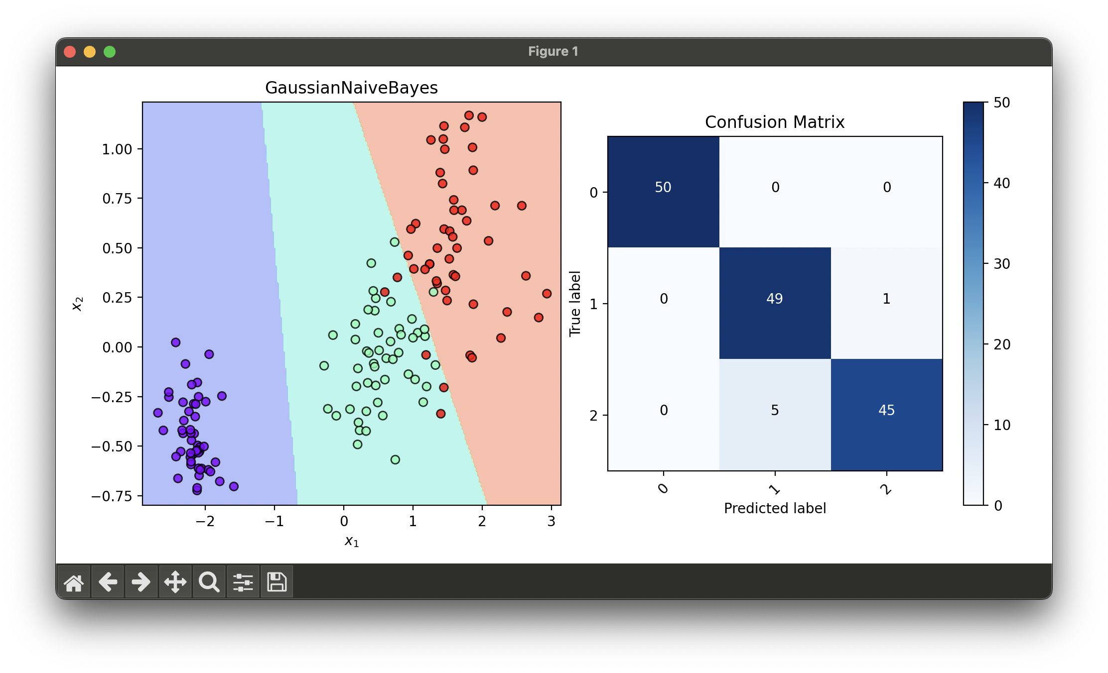
Test with iris flower dataset and transform via LDA:

from luma.classifier.naive_bayes import GaussianNaiveBayes
from luma.preprocessing.scaler import StandardScaler
from luma.reduction.linear import LDA
from luma.model_selection.split import TrainTestSplit
from luma.visual.evaluation import DecisionRegion, ConfusionMatrix

import numpy as np
import matplotlib.pyplot as plt
from sklearn.datasets import load_iris


X, y = load_iris(return_X_y=True)

X_train, X_test, y_train, y_test = TrainTestSplit(X, y,
                                                  test_size=0.2,
                                                  random_state=42).get

sc = StandardScaler()
X_train_std = sc.fit_transform(X_train)
X_test_std = sc.fit_transform(X_test)

lda = LDA(n_components=2)
X_train_lda = lda.fit_transform(X_train_std, y_train)
X_test_lda = lda.transform(X_test_std)

gnb = GaussianNaiveBayes()
gnb.fit(X_train_lda, y_train)

X_concat = np.concatenate((X_train_lda, X_test_lda))
y_concat = np.concatenate((y_train, y_test))

fig = plt.figure(figsize=(10, 5))
ax1 = fig.add_subplot(1, 2, 1)
ax2 = fig.add_subplot(1, 2, 2)

dec = DecisionRegion(gnb, X_concat, y_concat)
dec.plot(ax=ax1)

conf = ConfusionMatrix(y_concat, gnb.predict(X_concat))
conf.plot(ax=ax2, show=True)

Applications and Use Cases

Gaussian Naive Bayes is utilized across various domains:

• Text Classification: Despite its simplicity, it performs well for spam filtering and sentiment analysis.
• Medical Diagnosis: Predicting the likelihood of diseases based on patient test results.
• Financial Forecasting: Assessing the risk of loan default based on historical financial data.

Strengths and Limitations

• Strengths
  • Efficient and easy to implement.
  • Performs well in multi-class classification.
  • Requires a small amount of training data to estimate the necessary parameters.
• Limitations
  • Assumes independence of features, which often does not hold true in real-world data.
  • The Gaussian assumption may not accurately represent the data distribution for all features.

Advanced Topics and Further Reading

For those interested in exploring beyond the basics of Gaussian Naive Bayes, consider investigating:

• Kernel Naive Bayes: Extends Naive Bayes to handle data that is not linearly separable by applying kernel methods.
• Comparative studies on Naive Bayes variants: Understanding the performance of Gaussian Naive Bayes in comparison to other variants like Multinomial and Bernoulli Naive Bayes.

References

1. McCallum, Andrew, and Kamal Nigam. "A comparison of event models for Naive Bayes text classification." AAAI-98 workshop on learning for text categorization. Vol. 752. No. 1. 1998.
2. Rish, Irina. "An empirical study of the naive Bayes classifier." IJCAI 2001 workshop on empirical methods in artificial intelligence. Vol. 3. No. 22. 2001.
3. John, George H., and Pat Langley. "Estimating continuous distributions in Bayesian classifiers." Proceedings of the Eleventh conference on Uncertainty in artificial intelligence. Morgan Kaufmann Publishers Inc., 1995.