Softmax Regression

Introduction

Softmax Regression, commonly known as Multinomial Logistic Regression, is a generalization of logistic regression that allows for a response variable to model multiple classes. It is particularly useful in scenarios where the outcome can assume more than two categories, making it a staple algorithm in the field of machine learning for handling multi-class classification problems.

Background and Theory

Unlike binary logistic regression, which models the probability of a single binary outcome, softmax regression models the probabilities of multiple classes based on a single set of features. It employs the softmax function to map the cumulative linear scores of the features to probabilities that sum to one across all classes. The core principle behind softmax regression is to predict a multinomial probability distribution for each observation.

How the Algorithm Works

Steps

1. Score Calculation: Compute a score for each class using a linear function of the input features. This involves multiplying the feature vector for each observation by a weight matrix and adding a bias vector.
2. Softmax Function Application: Apply the softmax function to the calculated scores to convert them into probabilities. The softmax function is what differentiates softmax regression from other types of regression, ensuring that the output probabilities are non-negative and sum to one.
3. Optimization: The parameters (weights and biases) are optimized using an objective function, typically cross-entropy loss, through an iterative process such as gradient descent.

Mathematical Formulation

Let $\mathbf{x}$ be an input feature vector, $\mathbf{W}$ be the weight matrix, and $\mathbf{b}$ be the bias vector. For $K$ classes, the score for class $k$ is given by:

where $\mathbf{w}_k$ is the weight vector corresponding to class $k$, and $b_k$ is the bias term for class $k$.

The softmax function is then applied to the vector of scores $\mathbf{z}$ to obtain the probability distribution over the $K$ classes:

where $P(y=k|\mathbf{x})$ is the probability that $\mathbf{x}$ belongs to class $k$.

Regularization

To prevent overfitting, regularization techniques can be incorporated into the optimization process. L1 and L2 regularizations are common choices, adding a penalty term to the loss function based on the magnitude of the coefficients.

• L1 Regularization: Adds a penalty equal to the absolute value of the magnitude of coefficients, encouraging sparsity in the model parameters.
• L2 Regularization: Adds a penalty equal to the square of the magnitude of coefficients, penalizing large values of parameters.

The regularized loss function can be written as:

where $\|\mathbf{W}\|_F^2$ denotes the Frobenius norm of the weight matrix, $\lambda$ is the regularization strength, and $y_{ik}$ is the indicator variable that is 1 if the class label $y_i$ is $k$ and 0 otherwise.

Optimization Process

The optimization of the softmax regression model involves minimizing the regularized loss function. This is typically achieved through iterative optimization algorithms such as gradient descent or its variants (e.g., stochastic gradient descent, Adam). The gradient of the loss function with respect to the weight matrix $\mathbf{W}$ is computed and used to update the parameters in the direction that minimally decreases the loss.

Implementation

Parameters

• leraning_rate: float, default = 0.01
  Step size of the gradient descent update
  
• max_iter: int, default = 100
  Number of iteration
  
• l1_ratio: float, default = 0.5
  Balancing parameter of ‘elastic-net’ regularization
  
• alpha: float, default = 0.01
  Regularization strength
  
• regularization: Literal['l1', 'l2', 'elastic-net'], default = None
  Regularization method (’None’ for no regularization)

Examples

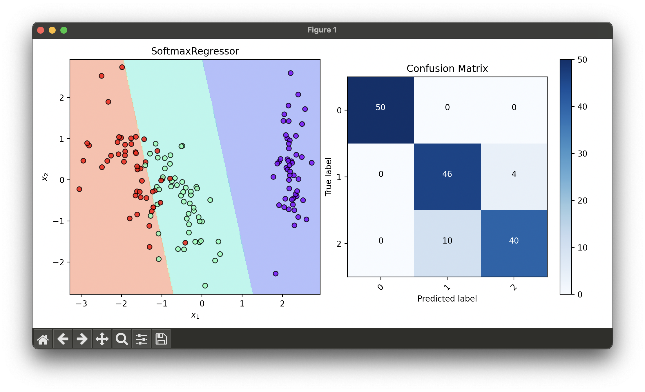
Test with iris flower dataset and tune hyperparameters via RandomizedSearchCV:

from luma.classifier.logistic import SoftmaxRegressor
from luma.preprocessing.scaler import StandardScaler
from luma.model_selection.split import TrainTestSplit
from luma.model_selection.search import RandomizedSearchCV
from luma.reduction.linear import PCA
from luma.visual.evaluation import DecisionRegion, ConfusionMatrix

from sklearn.datasets import load_iris
import matplotlib.pyplot as plt
import numpy as np


X, y = load_iris(return_X_y=True)

X_train, X_test, y_train, y_test = TrainTestSplit(X, y,
                                                  test_size=0.2, 
                                                  random_state=42).get

sc = StandardScaler()
X_train_std = sc.fit_transform(X_train)
X_test_std = sc.fit_transform(X_test)

pca = PCA(n_components=2)
X_train_pca = pca.fit_transform(X_train_std)
X_test_pca = pca.fit_transform(X_test_std)

param_dist = {'learning_rate': np.logspace(-3, -1, 5),
              'max_iter': [100],
              'l1_ratio': np.linspace(0, 1, 5),
              'alpha': np.logspace(-3, 2, 5),
              'regularization': ['l1', 'l2', 'elastic-net']}

rand = RandomizedSearchCV(estimator=SoftmaxRegressor(),
                          param_dist=param_dist,
                          max_iter=100,
                          cv=5,
                          refit=True,
                          random_state=42)

rand.fit(X_train_pca, y_train)
soft_best = rand.best_model

fig = plt.figure(figsize=(10, 5))
ax1 = fig.add_subplot(1, 2, 1)
ax2 = fig.add_subplot(1, 2, 2)

X_trans = np.concatenate((X_train_pca, X_test_pca))
y_trans = np.concatenate((y_train, y_test))

dec = DecisionRegion(soft_best, X_trans, y_trans)
dec.plot(ax=ax1)

conf = ConfusionMatrix(y_trans, soft_best.predict(X_trans))
conf.plot(ax=ax2, show=True)

# Best params: {
#     'learning_rate': 0.1, 
#     'max_iter': 100, 
#     'l1_ratio': 1.0, 
#     'alpha': 0.01778279410038923, 
#     'regularization': 'l1'
# } 
# Best score: 0.9416666666666667

Applications and Use Cases

Softmax regression is versatile and can be applied to a wide range of multi-class classification problems, including but not limited to:

• Image classification, where each image is categorized into one of several classes.
• Language processing tasks, such as part-of-speech tagging or named entity recognition.
• Medical diagnosis, classifying patient outcomes into multiple possible diagnoses.

Strengths and Limitations

• Strengths
  • Capable of handling multiple classes directly.
  • Provides probabilities for each class, offering interpretability regarding class membership.
  • Efficient and scalable to large datasets.
• Limitations
  • Assumes independence among features.
  • Linear decision boundaries may not capture complex relationships in the data.
  • Susceptible to overfitting, especially with high-dimensional data, necessitating the use of regularization.

Advanced Topics and Further Reading

Further exploration into softmax regression can delve into topics such as:

• The integration of softmax regression in neural network architectures, particularly in the output layer for classification tasks.
• The comparison and contrast with other multi-class classification strategies, such as one-vs-rest (OvR) logistic regression.
• Advanced optimization techniques that improve upon traditional gradient descent for faster convergence and efficiency in training large-scale models.

References

1. Bishop, Christopher M. "Pattern Recognition and Machine Learning." Springer, 2006.
2. James, Gareth, Daniela Witten, Trevor Hastie, and Robert Tibshirani. "An Introduction to Statistical Learning: with Applications in R." Springer, 2013.
3. Murphy, Kevin P. "Machine Learning: A Probabilistic Perspective." The MIT Press, 2012.
4. Goodfellow, Ian, Yoshua Bengio, and Aaron Courville. "Deep Learning." The MIT Press, 2016.