Kernel Discriminant Analysis Classifier

Introduction

Kernel Discriminant Analysis (KDA), also known as Kernel Fisher Discriminant Analysis, is a nonlinear generalization of Linear Discriminant Analysis (LDA) that uses kernel methods to project linearly inseparable data into a higher-dimensional space where it becomes linearly separable. This technique is particularly useful for complex datasets where the relationship between classes cannot be captured by linear decision boundaries.

Background and Theory

The fundamental concept behind KDA is the use of a kernel function to implicitly map the input data into a high-dimensional feature space. In this feature space, classical LDA is then applied to find linear decision boundaries. The beauty of KDA lies in its ability to handle nonlinear relationships without the need for explicit computation in the high-dimensional space, thanks to the kernel trick.

The choice of kernel (e.g., polynomial, radial basis function, sigmoid) plays a crucial role in the performance of KDA, as it determines the nature of the feature space and thus how well the data can be separated.

How the Algorithm Works

Steps

1. Select a kernel function and map the data to a higher-dimensional space

   The kernel function computes the inner product between data points in the feature space without explicitly performing the transformation.

2. Compute the between-class and within-class scatter matrices in the feature space

   These matrices characterize the distribution of the transformed data with respect to class separability.

3. Solve for the optimal projection vectors

   This involves finding the eigenvectors that maximize the ratio of the between-class scatter to the within-class scatter in the feature space.

4. Project data points onto the found vectors for classification

   This step involves using the projection vectors to transform data points into a space where they can be linearly separated.

Mathematical Formulation

The objective of KDA is to maximize the following criterion:

where $S_B$ and $S_W$ are the between-class and within-class scatter matrices in the feature space, respectively. The solution involves solving a generalized eigenvalue problem in the context of the selected kernel function.

Implementation

Parameters

• deg: int, default = 2
  Polynomial degree of ‘poly’ kernel
  
• gamma: float, default = 1.0
  Shape parameter of ‘rbf’, ‘sigmoid’, ‘laplacian’ kernels
  
• alpha: float, default = 1.0
  Shape parameter of ‘rbf’, ‘sigmoid’, ‘laplacian’ kernels
  
• coef: float, default = 1.0
  Additional coefficient of ‘poly’ and ‘sigmoid’ kernels
  
• kernel: KernelUtil.func_type, default = ‘rbf’
  Type of kernel functions
  

Examples

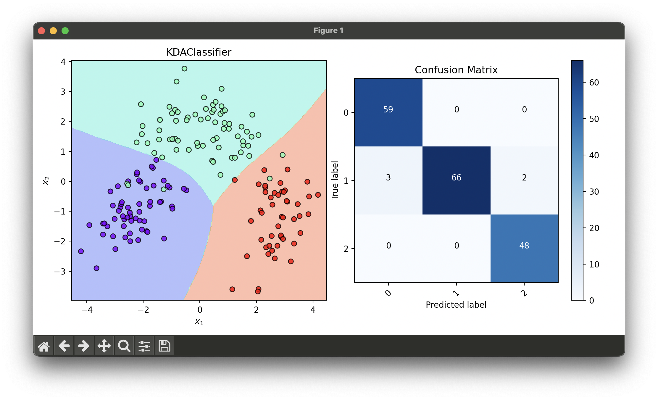
Test with wine dataset and tune hyperparameters via RandomizedSearchCV

from luma.classifier.discriminant import KDAClassifier
from luma.preprocessing.scaler import StandardScaler
from luma.model_selection.split import TrainTestSplit
from luma.model_selection.search import RandomizedSearchCV
from luma.reduction.linear import PCA
from luma.visual.evaluation import DecisionRegion, ConfusionMatrix

from sklearn.datasets import load_wine
import matplotlib.pyplot as plt
import numpy as np


X, y = load_wine(return_X_y=True)

X_train, X_test, y_train, y_test = TrainTestSplit(X, y,
                                                  test_size=0.2, 
                                                  random_state=42).get

sc = StandardScaler()
X_train_std = sc.fit_transform(X_train)
X_test_std = sc.fit_transform(X_test)

pca = PCA(n_components=2)
X_train_pca = pca.fit_transform(X_train_std)
X_test_pca = pca.fit_transform(X_test_std)

param_dist = {'deg': range(3, 10),
              'gamma': np.logspace(-3, 1, 5),
              'kernel': ['rbf', 'sigmoid', 'laplacian']}

rand = RandomizedSearchCV(estimator=KDAClassifier(),
                          param_dist=param_dist,
                          max_iter=100,
                          cv=5,
                          refit=True,
                          random_state=42)

rand.fit(X_train_pca, y_train)
kda_best = rand.best_model

fig = plt.figure(figsize=(10, 5))
ax1 = fig.add_subplot(1, 2, 1)
ax2 = fig.add_subplot(1, 2, 2)

X_trans = np.concatenate((X_train_pca, X_test_pca))
y_trans = np.concatenate((y_train, y_test))

dec = DecisionRegion(kda_best, X_trans, y_trans)
dec.plot(ax=ax1)

conf = ConfusionMatrix(y_trans, kda_best.predict(X_trans))
conf.plot(ax=ax2, show=True)

# Best params: {'deg': 7, 'gamma': 10.0, 'kernel': 'rbf'} 
# Best Score: 0.9728110599078341

Applications and Use Cases

KDA is widely used in fields such as bioinformatics, image recognition, and speech analysis, where the data exhibit complex patterns that are not linearly separable. Its ability to capture nonlinear relationships makes it particularly useful for tasks like facial recognition and gene expression classification.

Strengths and Limitations

• Strengths
  • Can capture complex nonlinear relationships in the data.
  • Flexible in terms of the choice of kernel function to suit different data characteristics.
  • Effective for high-dimensional data analysis.
• Limitations
  • Selection of an appropriate kernel function and its parameters can be challenging.
  • Computationally intensive, especially for large datasets.
  • May suffer from overfitting in the presence of noise or irrelevant features.

Advanced Topics and Further Reading

Further exploration into KDA can involve the study of different kernel functions and their impact on model performance, techniques for parameter optimization (e.g., cross-validation), and comparison with other kernel-based methods such as Support Vector Machines (SVMs) and Kernel Principal Component Analysis (KPCA).

References

1. Mika, S., Ratsch, G., Weston, J., Scholkopf, B., & Mullers, K.R. (1999). "Fisher Discriminant Analysis with Kernels." Neural Networks for Signal Processing IX: Proceedings of the 1999 IEEE Signal Processing Society Workshop.
2. Scholkopf, B., & Smola, A. J. (2002). Learning with Kernels: Support Vector Machines, Regularization, Optimization, and Beyond. MIT Press.
3. Duda, R. O., Hart, P. E., & Stork, D. G. (2001). Pattern Classification (2nd ed.). Wiley-Interscience.