Logistic Regression

Introduction

Logistic Regression is a statistical method for analyzing datasets in which there are one or more independent variables that determine an outcome. The outcome is measured with a dichotomous variable (in which there are only two possible outcomes). It is used extensively in various fields, including machine learning, for binary classification problems. Logistic regression estimates the probabilities using a logistic function, which is the cumulative logistic distribution.

Background and Theory

At its core, Logistic Regression is a linear regression model adapted to scenarios where the dependent variable is categorical. The key concept behind logistic regression is the use of the logistic function, also known as the sigmoid function, which takes any real-valued number and maps it into a value between 0 and 1, making it suitable for estimating probabilities. The logistic function is defined as:

where $z$ is the input to the function, $e$ is the base of the natural logarithm, and $\sigma(z)$ is the output between 0 and 1.

How the Algorithm Works

Steps

1. Model Construction: Construct the regression model to predict the log-odds of the dependent variable, typically using a linear combination of the independent variables.
2. Estimation of Coefficients: Use Maximum Likelihood Estimation (MLE) to estimate the coefficients of the model. This involves optimizing the logistic likelihood function to find the best parameters.
3. Prediction: For a new set of inputs, predict the log-odds of the outcome, convert these log-odds to probabilities using the logistic function, and make predictions based on these probabilities.

Mathematical Formulation

The logistic regression model is formulated as follows:

where $p$ is the probability of the outcome being 1, $X_i$ are the independent variables, and $\beta_i$ are the coefficients to be estimated.

The probability $p$ can be expressed using the logistic function as:

Regularization

Regularization techniques are used to prevent overfitting by penalizing large coefficients in the model. There are two main types of regularization:

• L1 Regularization (Lasso): Adds the absolute value of coefficients to the loss function. It can lead to some coefficients being exactly zero, providing a form of feature selection. The cost function with L1 regularization is:
  $J(\theta) = -\frac{1}{m} \sum_{i=1}^{m} [y^{(i)} \log(h_\theta(x^{(i)})) + (1 - y^{(i)}) \log(1 - h_\theta(x^{(i)}))] + \lambda \sum_{j=1}^{n} |\theta_j|$
• L2 Regularization (Ridge): Adds the square of the value of coefficients to the loss function, penalizing large coefficients but not setting them to zero. The cost function with L2 regularization is:
  $J(\theta) = -\frac{1}{m} \sum_{i=1}^{m} [y^{(i)} \log(h_\theta(x^{(i)})) + (1 - y^{(i)}) \log(1 - h_\theta(x^{(i)}))] + \lambda \sum_{j=1}^{n} \theta_j^2$

where $m$ is the number of observations, $y^{(i)}$ is the outcome for the $i$-th observation, $h_\theta(x^{(i)})$ is the hypothesis function, $\lambda$ is the regularization parameter, and $\theta_j$ are the coefficients.

Optimization

The coefficients of the logistic regression model are typically found using optimization algorithms such as Gradient Descent. The goal is to minimize the cost function $J(\theta)$, which measures the difference between the predicted probabilities and the actual outcomes.

• Gradient Descent: An iterative optimization algorithm used to minimize the cost function by iteratively moving in the direction of steepest descent as defined by the negative of the gradient.

The update rule for gradient descent is:

where $\alpha$ is the learning rate, and ${\partial J(\theta)}/{\partial \theta_j}$ is the partial derivative of the cost function with respect to the $j$-th parameter.

Implementation

Parameters

• leraning_rate: float, default = 0.01
  Step size of the gradient descent update
  
• max_iter: int, default = 100
  Number of iteration
  
• l1_ratio: float, default = 0.5
  Balancing parameter of ‘elastic-net’ regularization
  
• alpha: float, default = 0.01
  Regularization strength
  
• regularization: Literal['l1', 'l2', 'elastic-net'], default = None
  Regularization method (’None’ for no regularization)

Examples

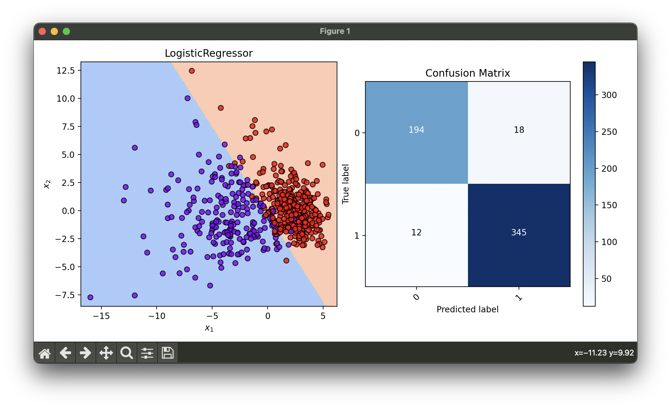
Test with breast cancer dataset and tune hyperparameters via RandomizedSearchCV:

from luma.classifier.logistic import LogisticRegressor
from luma.preprocessing.scaler import StandardScaler
from luma.reduction.linear import PCA
from luma.model_selection.split import TrainTestSplit
from luma.model_selection.search import RandomizedSearchCV
from luma.visual.evaluation import DecisionRegion, ConfusionMatrix

from sklearn.datasets import load_breast_cancer
import numpy as np
import matplotlib.pyplot as plt


X, y = load_breast_cancer(return_X_y=True)

X_train, X_test, y_train, y_test = TrainTestSplit(X, y,
                                                  test_size=0.2,
                                                  random_state=42).get

sc = StandardScaler()
X_train_std = sc.fit_transform(X_train)
X_test_std = sc.fit_transform(X_test)

pca = PCA(n_components=2)
X_train_pca = pca.fit_transform(X_train_std)
X_test_pca = pca.fit_transform(X_test_std)

param_dist = {'learning_rate': np.logspace(-3, -1, 5),
              'max_iter': [100],
              'l1_ratio': np.linspace(0, 1, 5),
              'alpha': np.logspace(-2, 2, 5),
              'regularization': ['l1', 'l2', 'elastic-net']}

rand = RandomizedSearchCV(estimator=LogisticRegressor(),
                          param_dist=param_dist,
                          max_iter=100,
                          cv=5,
                          refit=True,
                          random_state=42)

rand.fit(X_train_pca, y_train)
log_best = rand.best_model

X_concat = np.concatenate((X_train_pca, X_test_pca))
y_concat = np.concatenate((y_train, y_test))

fig = plt.figure(figsize=(10, 5))
ax1 = fig.add_subplot(1, 2, 1)
ax2 = fig.add_subplot(1, 2, 2)

dec = DecisionRegion(log_best, X_concat, y_concat)
dec.plot(ax=ax1)

conf = ConfusionMatrix(y_concat, log_best.predict(X_concat))
conf.plot(ax=ax2, show=True)

# Best params: {
#     'learning_rate': 0.01, 
#     'max_iter': 100, 
#     'l1_ratio': 0.75, 
#     'alpha': 0.01, 
#     'regularization': 'l2'
# }
# Best score: 0.9495222169135212

Applications and Use Cases

Logistic Regression is widely used in various fields such as:

• Medical Fields: Predicting the likelihood of a patient having a disease based on observed characteristics.
• Financial Services: Credit scoring to predict loan defaulters.
• Marketing: Predicting customer churn in subscription services.
• Social Sciences: Analyzing election outcomes based on demographic data.

Strengths and Limitations

• Strengths
  • Simple to implement and interpret.
  • Efficient to train.
  • Outputs have a nice probabilistic interpretation.
  • Can be regularized to avoid overfitting.
• Limitations
  • Assumes a linear relationship between the log-odds of the outcome and the independent variables.
  • Not suitable for complex relationships or non-linear problems.
  • Sensitive to unbalanced data.

Advanced Topics and Further Reading

• Regularization in Logistic Regression: An in-depth look at L1 and L2 regularization techniques.
• Multinomial and Ordinal Logistic Regression: Extensions of logistic regression for multi-class classification problems.
• Optimization Techniques: Detailed exploration of optimization algorithms used in logistic regression, like Stochastic Gradient Descent (SGD).

References

1. D. W. Hosmer Jr, S. Lemeshow, and R. X. Sturdivant, "Applied Logistic Regression," 3rd ed. Wiley, 2013.
2. J. H. Friedman, T. Hastie, and R. Tibshirani, "The elements of statistical learning," Springer series in statistics Springer, Berlin, 2001.
3. S. Menard, "Applied Logistic Regression Analysis," Sage, 2002.
4. E. P. Cramer, "The Sage Dictionary of Statistics: A Practical Resource for Students in the Social Sciences," Sage, 2004.