Regularized Discriminant Analysis Classifier

Introduction

Regularized Discriminant Analysis (RDA) is an extension of Quadratic Discriminant Analysis (QDA) and Linear Discriminant Analysis (LDA) that aims to improve classification accuracy by introducing a regularization parameter to the covariance matrices. This regularization helps to stabilize the estimates of the covariance matrices, particularly in scenarios where the number of features is close to or exceeds the number of observations, or when the data is highly collinear.

Background and Theory

RDA addresses some of the limitations of LDA and QDA by providing a compromise between the two. LDA assumes equal covariance matrices across classes, while QDA allows each class to have its own covariance matrix. RDA introduces a regularization parameter that adjusts the covariance matrices towards a common covariance matrix (as in LDA) or towards the identity matrix, thus controlling the model's complexity and preventing overfitting.

The core idea behind RDA is to blend the within-class covariance matrices of QDA with the pooled covariance matrix of LDA, along with a shrinkage parameter that regularizes the covariance matrices towards the identity matrix. This approach reduces the variance of the classifier and improves its performance on new, unseen data.

How the Algorithm Works

Steps

1. Calculate the pooled covariance matrix and the individual class covariance matrices

   Similar to LDA and QDA, compute these matrices based on the training data.

2. Apply regularization to the covariance matrices

   Adjust the covariance matrices by blending them with the pooled covariance matrix and the identity matrix, controlled by regularization parameters.

3. Compute the regularized discriminant function for each class

   Use the regularized covariance matrices and mean vectors to define the discriminant function.

4. Classify each data point

   Assign each data point to the class with the highest value of the discriminant function.

Mathematical Formulation

The regularized covariance matrix $\Sigma_{k}^{RDA}$ is given by:

where:

• $\Sigma_{k}$ is the covariance matrix for class $k$,
• $\Sigma_{P}$ is the pooled covariance matrix across all classes,
• $I$ is the identity matrix,
• $\alpha$ and $\gamma$ are regularization parameters controlling the blend between $\Sigma_{k}$, $\Sigma_{P}$, and $I$.

The discriminant function for RDA then becomes:

Implementation

Parameters

• alpha: float, default = 0.5
  Balancing parameter between the class-specific covariance matrices (0 for LDA-like, 1 for QDA-like approach)
  
• gamma: float, default = 0.5
  Shrinkage applied to the covariance matrices (0 for large shrinkage, i.e. max regularization)
  

Examples

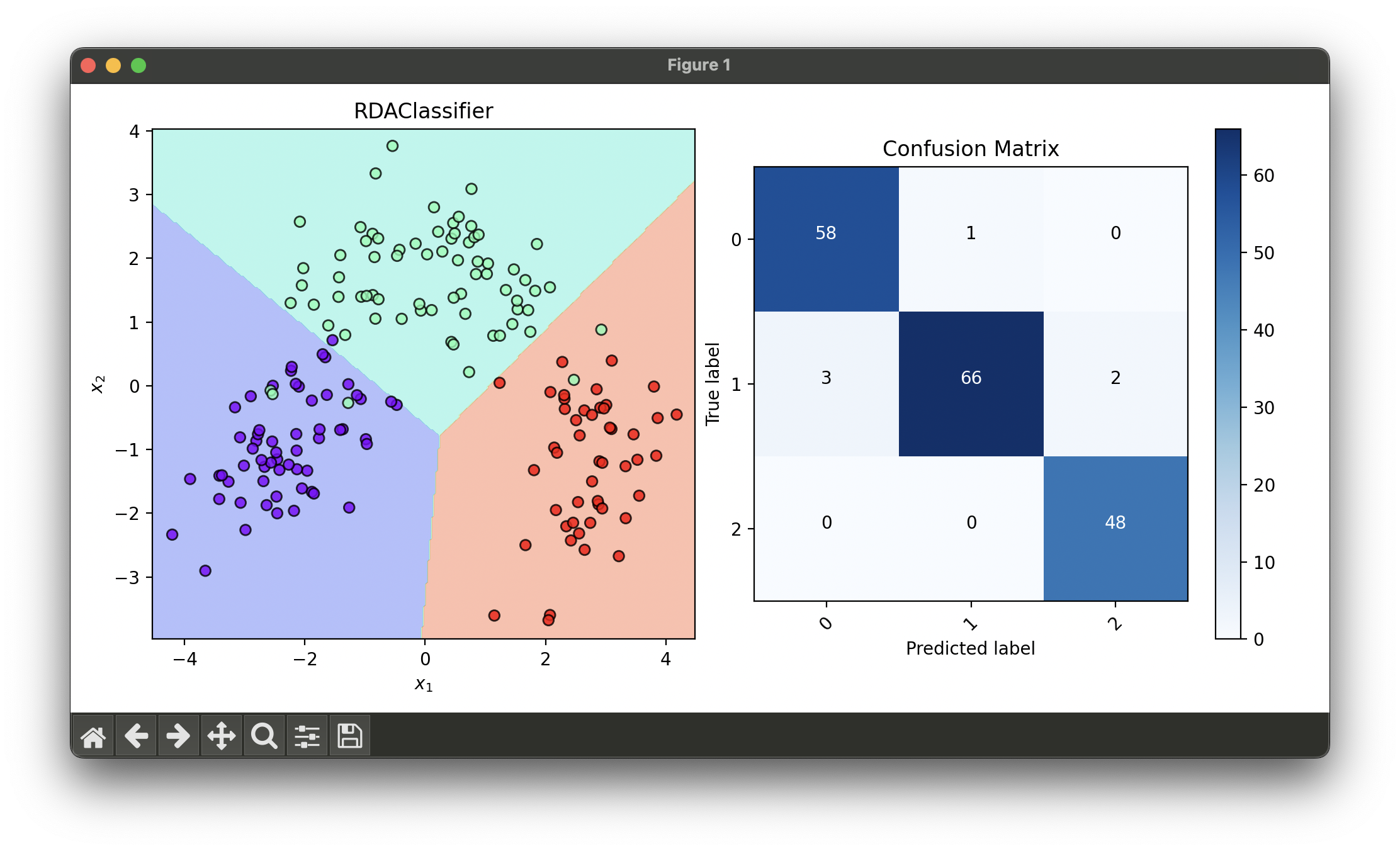
Test with wine dataset and tune hyperparameters via GridSearchCV

from luma.classifier.discriminant import RDAClassifier
from luma.preprocessing.scaler import StandardScaler
from luma.model_selection.split import TrainTestSplit
from luma.model_selection.search import GridSearchCV
from luma.reduction.linear import PCA
from luma.visual.evaluation import DecisionRegion, ConfusionMatrix

from sklearn.datasets import load_wine
import matplotlib.pyplot as plt
import numpy as np

X, y = load_wine(return_X_y=True)

X_train, X_test, y_train, y_test = TrainTestSplit(X, y,
                                                  test_size=0.2, 
                                                  random_state=42).get

sc = StandardScaler()
X_train_std = sc.fit_transform(X_train)
X_test_std = sc.fit_transform(X_test)

pca = PCA(n_components=2)
X_train_pca = pca.fit_transform(X_train_std)
X_test_pca = pca.fit_transform(X_test_std)

param_grid = {'alpha': np.linspace(0.01, 1, 5),
              'gamma': np.linspace(0.01, 1, 5)}

grid = GridSearchCV(estimator=RDAClassifier(),
                    param_grid=param_grid,
                    cv=5,
                    refit=True, 
                    random_state=42)

grid.fit(X_train_pca, y_train)
rda_best = grid.best_model

fig = plt.figure(figsize=(10, 5))
ax1 = fig.add_subplot(1, 2, 1)
ax2 = fig.add_subplot(1, 2, 2)

X_trans = np.concatenate((X_train_pca, X_test_pca))
y_trans = np.concatenate((y_train, y_test))

dec = DecisionRegion(rda_best, X_trans, y_trans)
dec.plot(ax=ax1)

conf = ConfusionMatrix(y_trans, rda_best.predict(X_trans))
conf.plot(ax=ax2, show=True)

# Best params: {'alpha': 0.01, 'gamma': 0.01}
# Best score: 0.965668202764977

Applications and Use Cases

RDA is used in situations where the dataset has a large number of features, in the presence of multicollinearity, or when the dataset contains outliers that may skew the covariance matrix. Its applications span various domains such as finance, genomics, and image recognition, where it helps in improving the robustness and accuracy of classification models.

Strengths and Limitations

• Strengths
  • Reduces the risk of overfitting by regularizing the covariance matrices.
  • More flexible and robust compared to LDA and QDA, especially in high-dimensional spaces.
  • Can handle situations where the number of features is larger than the number of samples.
• Limitations
  • The choice of regularization parameters is critical and may require cross-validation to optimize.
  • Can be computationally more intensive than LDA due to the additional regularization steps.
  • The effectiveness of regularization may vary depending on the underlying distribution of the data.

Advanced Topics and Further Reading

For further exploration, topics such as the selection of regularization parameters, comparison of RDA with other regularization techniques like ridge regression and lasso, and kernel-based methods for non-linear classification provide valuable insights into advanced machine learning strategies.

References

1. Friedman, J. (1989). "Regularized Discriminant Analysis." Journal of the American Statistical Association.
2. Hastie, T., Tibshirani, R., & Friedman, J. (2009). The Elements of Statistical Learning. New York: Springer.
3. McLachlan, G. J. (1992). Discriminant Analysis and Statistical Pattern Recognition. Wiley-Interscience.