Quadratic Discriminant Analysis Classifier

Introduction

Quadratic Discriminant Analysis (QDA) is a statistical technique used in pattern recognition and machine learning to classify datasets with two or more classes. Unlike its counterpart, Linear Discriminant Analysis (LDA), which assumes equal covariance matrices for all classes, QDA allows for each class to have its own covariance matrix. This flexibility makes QDA more suitable for datasets where the assumption of equal covariances does not hold, providing a more accurate classification by considering the specific distribution of each class.

Background and Theory

QDA is based on the Bayes theorem, which calculates the probability of a data point belonging to a particular class, given its features. The decision boundaries between classes in QDA are quadratic, which allows for more complex relationships between variables compared to the linear boundaries used in LDA.

The main theoretical underpinning of QDA is the assumption that the data from each class follow a multivariate normal (Gaussian) distribution with class-specific mean vectors and covariance matrices. This assumption allows for the modeling of the probability density function of each class, which is then used to compute the posterior probabilities required for classification.

How the Algorithm Works

Steps

1. Calculate the mean vectors and covariance matrices for each class

   For each class, compute the mean vector and covariance matrix based on the training data.

2. Compute the discriminant function for each class

   The discriminant function is a quadratic function of the input features, defined by the class mean vector, covariance matrix, and the prior probability of the class. The exact formulation is given in the mathematical formulation section.

3. Classify each data point

   For a given data point, evaluate the discriminant function for each class and assign the data point to the class with the highest function value.

Mathematical Formulation

The discriminant function for QDA is given by:

where:

• $x$ is the feature vector of the data point to be classified,
• $\mu_k$ is the mean vector of class $k$,
• $\Sigma_k$ is the covariance matrix of class $k$,
• $P(Y=k)$ is the prior probability of class $k$,
• $|\Sigma_k|$ is the determinant of $\Sigma_k$.

Implementation

Parameters

No paramters.

Examples

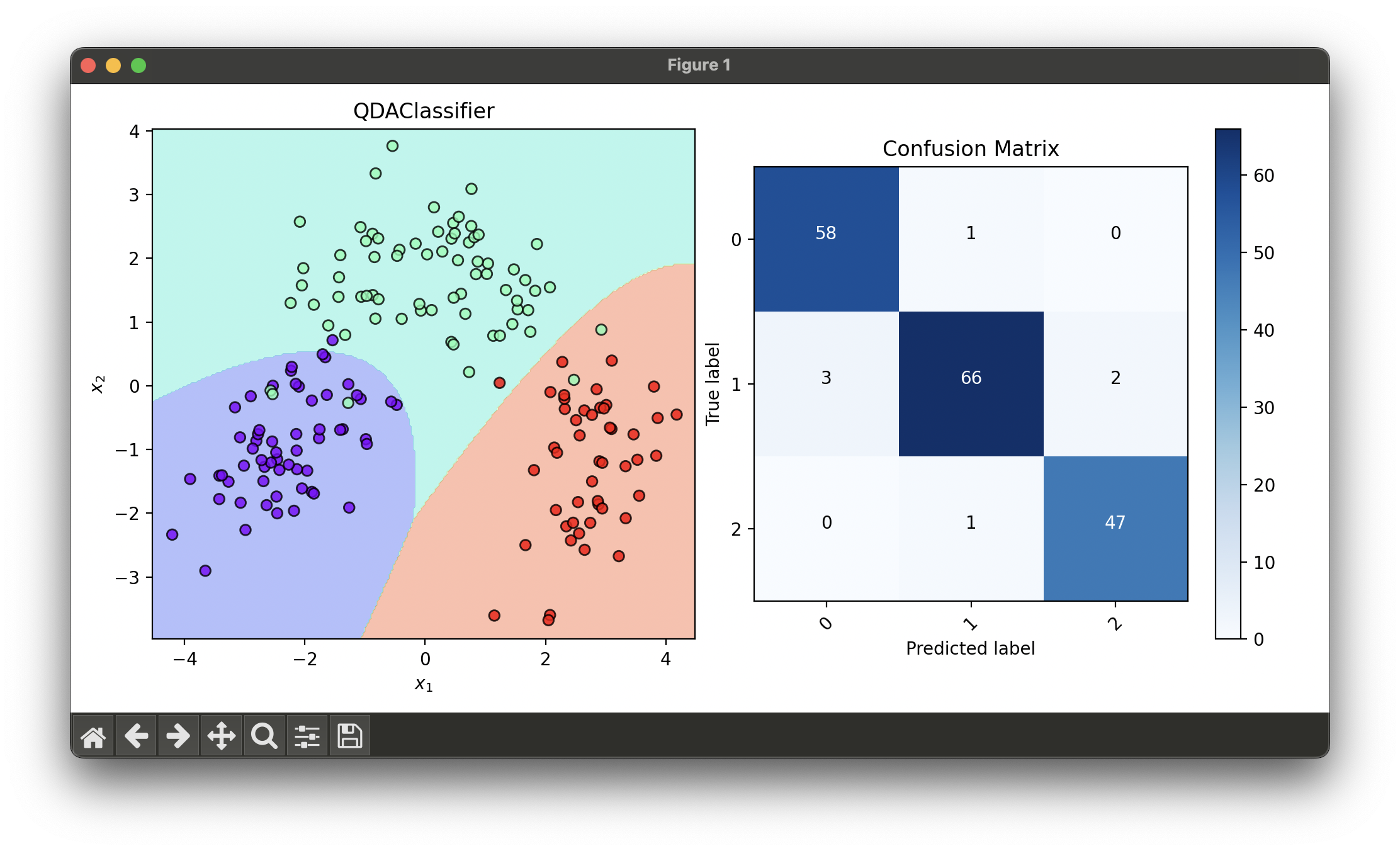
Test with wine dataset:

from luma.classifier.discriminant import QDAClassifier
from luma.preprocessing.scaler import StandardScaler
from luma.model_selection.split import TrainTestSplit
from luma.reduction.linear import PCA
from luma.visual.evaluation import DecisionRegion, ConfusionMatrix

from sklearn.datasets import load_wine
import matplotlib.pyplot as plt
import numpy as np


X, y = load_wine(return_X_y=True)

X_train, X_test, y_train, y_test = TrainTestSplit(X, y,
                                                  test_size=0.2, 
                                                  random_state=42).get

sc = StandardScaler()
X_train_std = sc.fit_transform(X_train)
X_test_std = sc.fit_transform(X_test)

pca = PCA(n_components=2)
X_train_pca = pca.fit_transform(X_train_std)
X_test_pca = pca.fit_transform(X_test_std)

qda = QDAClassifier()
qda.fit(X_train_pca, y_train)

fig = plt.figure(figsize=(10, 5))
ax1 = fig.add_subplot(1, 2, 1)
ax2 = fig.add_subplot(1, 2, 2)

X_trans = np.concatenate((X_train_pca, X_test_pca))
y_trans = np.concatenate((y_train, y_test))

dec = DecisionRegion(qda, X_trans, y_trans)
dec.plot(ax=ax1)

conf = ConfusionMatrix(y_trans, qda.predict(X_trans))
conf.plot(ax=ax2, show=True)

Applications and Use Cases

QDA is widely used in various fields such as finance, biology, and marketing for classification tasks. For example, in finance, QDA can be used to classify the risk levels of investments. In biology, it can help classify different species based on their features. In marketing, QDA can be used to segment customers into different groups based on purchasing behavior.

Strengths and Limitations

• Strengths
  • Can model complex relationships due to quadratic decision boundaries.
  • Flexible, as it does not assume equal covariance matrices across classes.
  • Effective in cases where the normality assumption for the data holds.
• Limitations
  • Prone to overfitting in cases of small sample size due to the estimation of covariance matrices.
  • Requires the inversion of covariance matrices, which can be computationally expensive for high-dimensional data.
  • The assumption of normal distribution may not hold for all real-world datasets.

Advanced Topics and Further Reading

For those interested in exploring beyond the basics of QDA, topics such as Regularized Discriminant Analysis (RDA) and comparison with other classification techniques like Support Vector Machines (SVMs) and neural networks offer further insights. Additionally, exploring kernel-based extensions of QDA can provide a deeper understanding of how to deal with non-linearly separable data.

References

1. James, G., Witten, D., Hastie, T., & Tibshirani, R. (2013). An Introduction to Statistical Learning. New York: Springer.
2. McLachlan, G. J. (2004). Discriminant Analysis and Statistical Pattern Recognition. Hoboken, NJ: Wiley-Interscience.
3. Bishop, C. M. (2006). Pattern Recognition and Machine Learning. New York: Springer.