Support Vector Classifier (Linear SVC)

Introduction

The Support Vector Classifier (Linear SVC) is a powerful linear model for classification tasks, derived from the Support Vector Machine (SVM) framework. It seeks to find the optimal separating hyperplane between classes in a high-dimensional space, maximizing the margin between the classes' nearest points, known as support vectors. This approach results in a classifier that is not only robust to outliers but also effective in high-dimensional spaces, making it widely applicable across various domains.

Background and Theory

SVC operates on the principle of structural risk minimization, focusing on both maximizing the margin between classes and minimizing classification error. The linear SVC specifically deals with linearly separable data, using a linear function to define the decision boundary. This simplicity allows for efficient computation while maintaining high performance for many tasks.

How the Algorithm Works

Steps

1. Feature Space Transformation: Map input features into a high-dimensional space (if necessary) where a linear separation is possible.
2. Optimization Problem Formulation: Formulate an optimization problem to find the hyperplane that maximizes the margin between the two classes.
3. Support Vector Identification: Identify the support vectors that are closest to the decision boundary.
4. Decision Function Construction: Construct a decision function based on the support vectors to classify new instances.

Mathematical Formulation

Given a dataset of $n$ points of the form $(\mathbf{x}_i, y_i)$ where $\mathbf{x}_i \in \mathbb{R}^p$ and $y_i \in \{-1, 1\}$, the goal is to find the optimal hyperplane $\mathbf{w}^T\mathbf{x} + b = 0$ that separates the classes. Here, $\mathbf{w}$ represents the weight vector and $b$ the bias.

The optimization problem can be stated as:

subject to the constraints:

This problem seeks to minimize $\|\mathbf{w}\|^2$ which is equivalent to maximizing the margin $2/\|\mathbf{w}\|$ between the classes, subject to the condition that all data points are classified correctly.

For non-linearly separable cases, a slack variable $\xi_i \geq 0$ is introduced for each data point to allow misclassification. The problem then includes a penalty term $C \sum \xi_i$ in the objective function, balancing the margin maximization and classification error:

subject to:

The parameter $C$ controls the trade-off between the slack variable penalty and the margin size, influencing the classifier's tolerance to misclassifications.

Implementation

Parameters

• C: float, default = 1.0 Regularization parameter
  
• batch_size: int, default = 100 Size of a single batch
  
• learning_rate: float, default = 0.001 Step-size of gradient descent update
  
• max_iter: int, default = 1000 Number of iteration
  

Examples

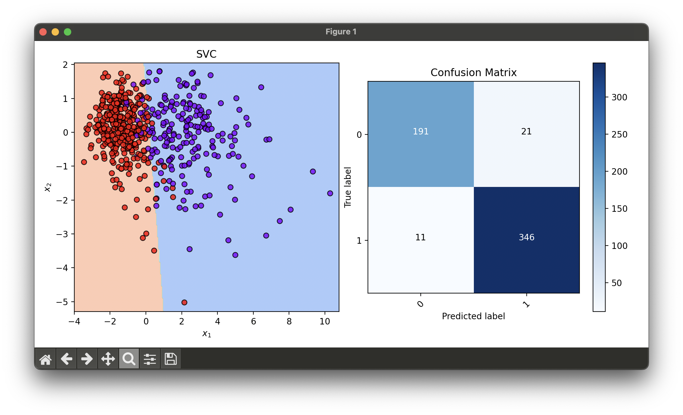
Test with breast cancer dataset and reduce dimensionality via LDA:

from luma.classifier.svm import SVC
from luma.preprocessing.scaler import StandardScaler
from luma.reduction.linear import LDA
from luma.model_selection.split import TrainTestSplit
from luma.model_selection.search import RandomizedSearchCV
from luma.visual.evaluation import DecisionRegion, ConfusionMatrix

from sklearn.datasets import load_breast_cancer
import matplotlib.pyplot as plt
import numpy as np


X, y = load_breast_cancer(return_X_y=True)

X_train, X_test, y_train, y_test = TrainTestSplit(X, y, 
                                                  test_size=0.2,
                                                  random_state=42).get

sc = StandardScaler()
X_train_std = sc.fit_transform(X_train)
X_test_std = sc.fit_transform(X_test)

lda = LDA(n_components=2)
X_train_tr = lda.fit_transform(X_train_std, y_train)
X_test_tr = lda.transform(X_test_std)

param_dist = {'C': np.logspace(-3, 2, 5),
              'learning_rate': np.logspace(-3, -0.5, 5)}

rand = RandomizedSearchCV(estimator=SVC(),
                          param_dist=param_dist,
                          max_iter=10,
                          cv=10,
                          refit=True,
                          random_state=42,
                          verbose=True)

rand.fit(X_train_tr, y_train)
svc_best = rand.best_model

X_concat = np.concatenate((X_train_tr, X_test_tr))
y_concat = np.concatenate((y_train, y_test))

fig = plt.figure(figsize=(10, 5))
ax1 = fig.add_subplot(1, 2, 1)
ax2 = fig.add_subplot(1, 2, 2)

dec = DecisionRegion(svc_best, X_concat, y_concat)
dec.plot(ax=ax1)

conf = ConfusionMatrix(y_concat, svc_best.predict(X_concat))
conf.plot(ax=ax2, show=True)

# Best params: {'C': 5.623413251903491, 'learning_rate': 0.01778279410038923}
# Best score: 0.9304575163398694

Applications and Use Cases

• Text Categorization: Efficiently classifying documents or emails into predefined categories.
• Image Classification: Identifying objects within images when the data can be linearly separated in feature space.
• Bioinformatics: Classifying biological samples into different categories based on their feature profiles.

Strengths and Limitations

• Strengths
  • High efficiency for linearly separable data, even in high-dimensional spaces.
  • Robustness against overfitting, especially in high-dimensional spaces, due to the margin maximization principle.
  • Flexibility through the regularization parameter $C$, allowing control over the trade-off between decision boundary margin and misclassification rate.
• Limitations
  • May perform poorly on highly non-linear data without kernel transformation.
  • Choice of the regularization parameter $C$ is critical and requires careful tuning.
  • Sensitive to feature scaling.

Advanced Topics and Further Reading

• Kernel Trick: For non-linearly separable data, the kernel trick can be applied to map inputs into higher-dimensional spaces where a linear separation is possible, without explicitly computing the transformation.
• Multi-Class Classification: Extending Linear SVC to handle more than two classes, either by constructing multiple binary classifiers (one-vs-rest) or by using methods that directly model multiple classes.
• Parameter Optimization: Techniques for selecting the optimal model parameters, including grid search and cross-validation.

References

1. Cortes, Corinna, and Vapnik, Vladimir. "Support-vector networks." Machine Learning 20.3 (1995): 273-297.
2. Boser, Bernhard E., Guyon, Isabelle M., and Vapnik, Vladimir N. "A training algorithm for optimal margin classifiers." Proceedings of the fifth annual workshop on Computational learning theory. 1992.
3. Schölkopf, Bernhard, and Smola, Alexander J. Learning with kernels: support vector machines, regularization, optimization, and beyond. MIT Press, 2002.
4. Hastie, Trevor, Tibshirani, Robert, and Friedman, Jerome. The Elements of Statistical Learning: Data Mining, Inference, and Prediction. Springer Series in Statistics. Springer, 2009.