AdaBoost Regressor

Introduction

AdaBoost (Adaptive Boosting) Regressor is an ensemble learning method specifically adapted for regression problems. Similar to its classification counterpart, it combines multiple weak regressors to create a strong regressor, focusing on instances that are difficult to predict. By iteratively adjusting the weights of training instances based on the current model's errors, AdaBoost Regressor aims to improve the model's prediction accuracy.

Background and Theory

AdaBoost for regression adapts the boosting methodology to fit continuous target values, rather than categorical ones. The principle remains the same: sequentially apply weak regressor models, adjust their influence on the final prediction based on their error, and thereby improve the robustness of the prediction over iterations.

Mathematical Formulation

Initial Setup

Given a dataset $D = \{(x_1, y_1), (x_2, y_2), \ldots, (x_n, y_n)\}$, where:

• $x_i$ represents the input features for instance $i$,
• $y_i \in \mathbb{R}$ represents the continuous target value for instance $i$,
• $n$ is the number of training instances.

The goal of AdaBoost Regressor is to construct a predictive model $F(x)$ that minimizes the expected value of a given loss function $L(y, F(x))$, where $L$ measures the difference between the predicted value $F(x)$ and the actual target value $y$.

Weight Initialization

Initially, each training instance is assigned an equal weight:

Iterative Process

For each iteration $t = 1, 2, \ldots, T$:

1. Train Weak Regressor: Train a weak regressor $h_t(x)$ using the training data weighted by $w_i^{(t)}$, where $w_i^{(t)}$ are the weights for the instances at iteration $t$.

2. Compute Error: Calculate the error $\epsilon_t$ of the weak regressor $h_t(x)$ using a loss function $L$:

   $\epsilon_t = \sum_{i=1}^{n} w_i^{(t)} L(y_i, h_t(x_i))$

3. Compute Regressor Weight: Determine the contribution $\alpha_t$ of $h_t(x)$ to the final model, often based on its error $\epsilon_t$. A common approach is to use:

   $\alpha_t = \frac{1}{2} \ln \left( \frac{1 - \epsilon_t}{\epsilon_t} \right)$

   This expression needs adaptation for regression tasks to ensure meaningful weight updates, especially since errors can vary more widely than in classification.

4. Update Weights: Update the weights of the instances for the next iteration $t+1$:

   $w_i^{(t+1)} = w_i^{(t)} \cdot \exp \left( -\alpha_t \cdot L(y_i, h_t(x_i)) \right)$

   where the function inside the $\exp$ might be adapted to ensure the weights increase for instances with larger errors and decrease for those with smaller errors.

5. Normalize Weights: Ensure the updated weights sum to 1:

   $w_i^{(t+1)} = \frac{w_i^{(t+1)}}{\sum_{j=1}^{n} w_j^{(t+1)}}$

Final Model

After $T$ iterations, the final model is a weighted sum of the weak regressors:

The objective is for $F(x)$ to closely approximate the true target values across the dataset, minimizing the overall loss.

Loss Function Adaptation

In practice, different loss functions can be used, and their choice impacts the performance of the AdaBoost Regressor. Common choices include:

• Squared Loss: $L(y, F(x)) = (y - F(x))^2$, which is sensitive to outliers but gives more weight to instances with larger errors.
• Absolute Loss: $L(y, F(x)) = |y - F(x)|$, which is less sensitive to outliers than squared loss.

The mathematical expressions provided above form the basis of the AdaBoost Regressor's algorithm, detailing the iterative process of adjusting instance weights, training weak regressors, and combining them into a final model aimed at minimizing the regression error.

Implementation

Parameters

• base_estimator: Estimator, default = DecisionTreeRegressor()
  Base estimator for training multiple models
  
• n_estimators: int, default = 100
  Number of base estimators to fit
  
• learning_rate: float, default = 1.0
  Step size of class weights($\vec\alpha$) update
  
• loss: Literal['linear', 'square', 'exp'], default = ‘linear’
  Type of loss function
  

Examples

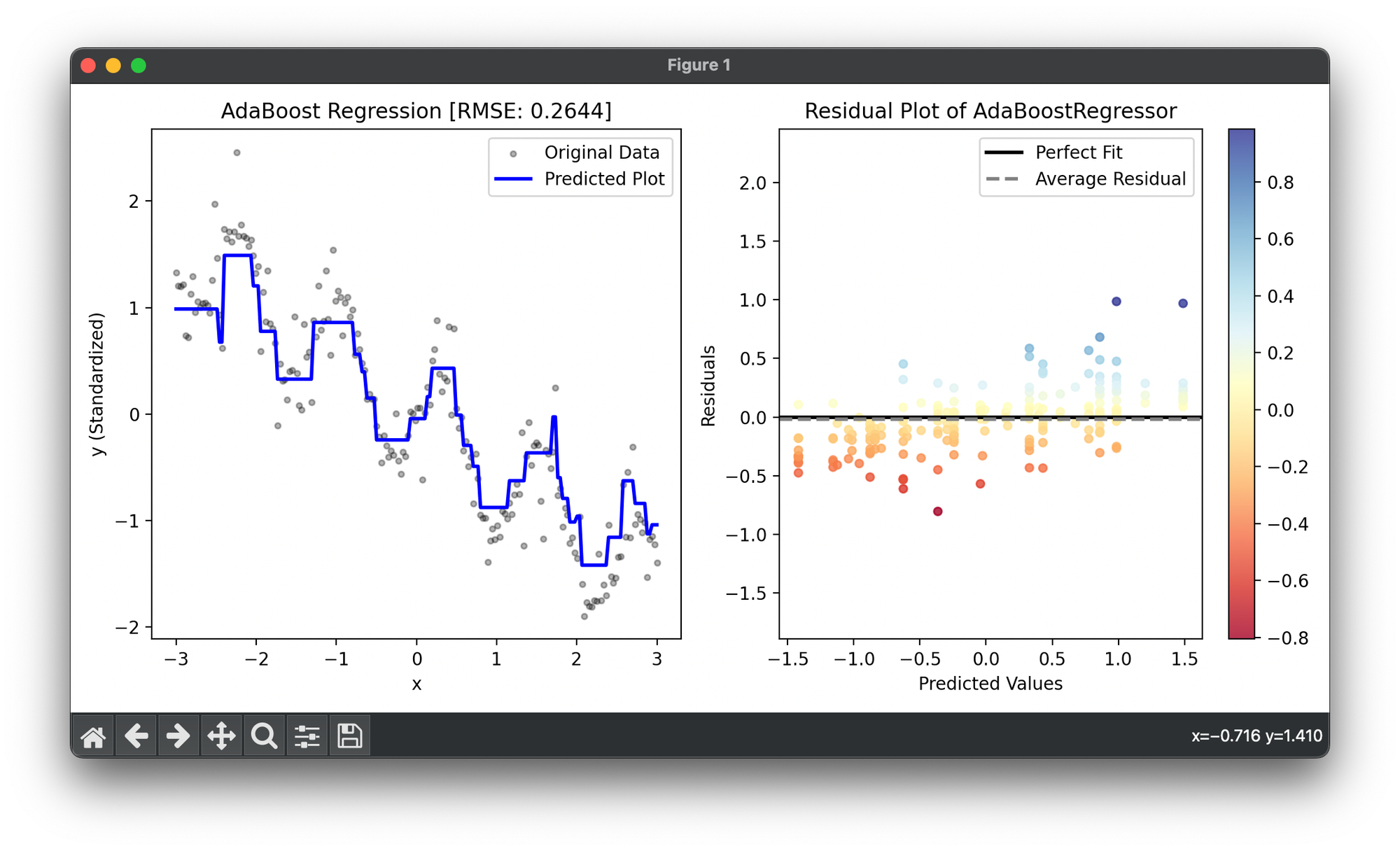
Test on synthesized dataset($y=\sin(5x)-x+\epsilon$):

from luma.ensemble.boost import AdaBoostRegressor
from luma.preprocessing.scaler import StandardScaler
from luma.metric.regression import RootMeanSquaredError
from luma.visual.evaluation import ResidualPlot

import matplotlib.pyplot as plt
import numpy as np

np.random.seed(42)

X = np.linspace(-3, 3, 200).reshape(-1, 1)
y = (np.sin(5 * X) - X).flatten() + 0.15 * np.random.randn(200)

rand_idx = np.random.choice(200, size=80)
y[rand_idx] += 0.75 * np.random.randn(80)

sc = StandardScaler()
y_trans = sc.fit_transform(y)

ada = AdaBoostRegressor(n_estimators=50,
                        learning_rate=1.0,
                        loss='linear',
                        max_depth=5)

ada.fit(X, y_trans)

y_pred = ada.predict(X)
score = ada.score(X, y_trans, metric=RootMeanSquaredError)

fig = plt.figure(figsize=(10, 5))
ax1 = fig.add_subplot(1, 2, 1)
ax2 = fig.add_subplot(1, 2, 2)

ax1.scatter(X, y_trans, s=10, c='black', alpha=0.3, label='Original Data')  
ax1.plot(X, y_pred, lw=2, c='blue', label='Predicted Plot')
ax1.legend()
ax1.set_xlabel('x')
ax1.set_ylabel('y (Standardized)')
ax1.set_title(f'AdaBoost Regression [RMSE: {score:.4f}]')

res = ResidualPlot(ada, X, y_trans)
res.plot(ax=ax2)
ax2.set_ylim(y_trans.min(), y_trans.max())

plt.tight_layout()
plt.show()

Applications

• Quantitative Prediction: Suitable for any regression task aiming to predict a numeric value, such as house prices, temperature forecasts, or stock market trends.
• Model Stacking: Can be used as part of a model stacking ensemble, where the outputs of several models are input into another model to improve predictions.
• Feature Importance Analysis: Similar to classification, AdaBoost regressor can be used to highlight the features most relevant to predicting the target variable.

Strengths and Limitations

Strengths

• Flexibility: Can be used with any regression model as the base learner.
• Automatic Feature Selection: Implicitly performs feature selection, giving more weight to the features that contribute most to the prediction.
• Robustness to Overfitting: Especially effective when the base regressors are simple, reducing the risk of overfitting complex datasets.

Limitations

• Sensitivity to Outliers: Just like in classification, the algorithm can be sensitive to noisy data and outliers because it focuses on correcting mispredictions.
• Computation Time: The sequential nature of the training process can lead to longer training times compared to some other algorithms.

Advanced Topics

• Loss Function Adaptations: Exploring different loss functions for regression, such as squared loss or absolute loss, and their impact on the performance of the AdaBoost regressor.
• AdaBoost.R2: A specific variant of AdaBoost designed for regression tasks, which adapts the algorithm to deal with continuous output spaces.

References

1. Drucker, Harris. "Improving regressors using boosting techniques." Proceedings of the fourteenth international conference on machine learning. 1997.
2. Solomatine, Dimitri P., and Dirk P. Van Den Boogaard. "Adaptive boosting (AB) for high-resolution rainfall-runoff modelling." Hydrological processes 19.14 (2005): 2729-2745.