Bagging Regressor

Introduction

The Bagging Regressor is an ensemble meta-algorithm designed to improve the stability and accuracy of machine learning algorithms through the process of bootstrapping the dataset and aggregating the predictions (hence the name Bagging, which stands for Bootstrap Aggregating). This technique is particularly useful in reducing variance, improving predictions, and preventing overfitting in regression models. Though it can be applied with various types of regression algorithms, it is most commonly used with decision trees.

Background and Theory

Bagging works by creating multiple copies of the original training dataset using bootstrap sampling, training a separate model on each copy, and then combining the outputs of these models into a single predictive model. The aggregation of predictions serves to reduce variance and avoid overfitting, especially in models that have high variance like decision trees.

Mathematical Foundations

Assuming a regression problem with a dataset $D = \{(x_1, y_1), (x_2, y_2), \ldots, (x_N, y_N)\}$, where $x_i$ represents the features and $y_i$ the target for the $i^\text{th}$ observation. Bagging involves the following steps:

1. Bootstrap Sampling: Generate $B$ bootstrap samples from the original dataset. Each sample, $D_b$, is generated by randomly selecting $N$ observations with replacement from $D$.
2. Model Training: Train a regression model $f_b$ on each bootstrap sample $D_b$.
3. Aggregation: The final bagging regressor prediction, $\hat{y}$, for a new instance with features $x$ is obtained by averaging the predictions from all individual regression models.

Mathematically, the prediction $\hat{y}$ of the bagging regressor for a new input $x$ is given by:

where $f_b(x)$ is the prediction of the $b^\text{th}$ model.

Variance Reduction

The effectiveness of bagging in reducing variance can be shown through its impact on the overall variance of the ensemble prediction. If we assume that the base models have a variance of $\sigma^2$ and are uncorrelated, the variance of the bagged estimator is:

This shows that the variance of the ensemble prediction decreases as the number of base models $B$ increases, which highlights the variance-reducing property of bagging.

Procedural Steps

1. Bootstrap the dataset: Generate $B$ different bootstrap samples from the original training dataset.
2. Train separate models: For each bootstrap sample, train a separate regression model.
3. Aggregate predictions: For a given test instance, the final prediction is obtained by averaging the predictions from all the individual models.

Implementation

Parameters

• base_estimator: Estimator, default = DecisionTreeRegressor()
  Base estimator for training multiple models
  
• n_estimators: int, default = 50
  Number of base estimators to fit
  
• max_samples: float int, default = 1.0
  Maximum number of data to sample (0~1 proportion)
  
• max_features: float int, default = 1.0
  Maximum number of features to sample (0~1 proporton)
  
• bootstrap: bool, default = True
  Whether to bootstrap data samples
  
• bootstrap_feature: bool, default = False
  Whether to bootstrap features
  

Examples

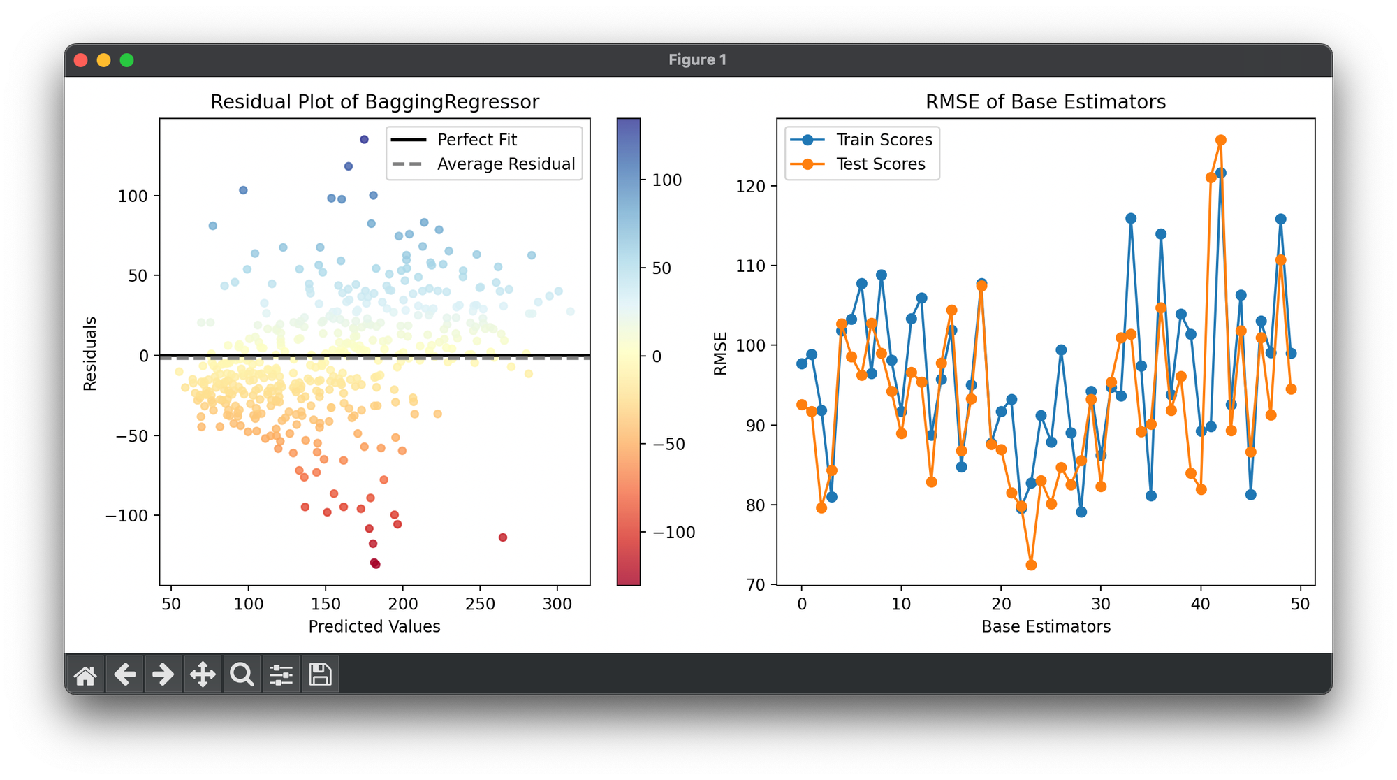
Test on diabetes dataset with DecisionTreeRegressor() as a base estimator:

from luma.ensemble.bagging import BaggingRegressor
from luma.preprocessing.scaler import StandardScaler
from luma.model_selection.split import TrainTestSplit
from luma.model_selection.search import RandomizedSearchCV
from luma.metric.regression import RootMeanSquaredError
from luma.visual.evaluation import ResidualPlot

from sklearn.datasets import load_diabetes
import matplotlib.pyplot as plt
import numpy as np

X, y = load_diabetes(return_X_y=True)

X_train, X_test, y_train, y_test = TrainTestSplit(X, y,
                                                  test_size=0.3,
                                                  random_state=42).get

sc = StandardScaler()
X_train_std = sc.fit_transform(X_train)
X_test_std = sc.fit_transform(X_test)

param_dist = {'n_estimators': [10, 20, 50],
              'max_samples': np.linspace(0.5, 1.0, 5),
              'max_features': np.linspace(0.5, 1.0, 5),
              'bootstrap': [True, False],
              'bootstrap_feature': [True, False],
              'random_state': [42]}

rand = RandomizedSearchCV(estimator=BaggingRegressor(),
                          param_dist=param_dist,
                          cv=5,
                          max_iter=10,
                          metric=RootMeanSquaredError,
                          maximize=False, 
                          refit=True,
                          random_state=42,
                          verbose=True)

rand.fit(X_train_std, y_train)
bag_best: BaggingRegressor = rand.best_model

X_cat = np.concatenate((X_train_std, X_test_std))
y_cat = np.concatenate((y_train, y_test))

fig = plt.figure(figsize=(11, 5))
ax1 = fig.add_subplot(1, 2, 1)
ax2 = fig.add_subplot(1, 2, 2)

res = ResidualPlot(bag_best, X_cat, y_cat)
res.plot(ax=ax1)

train_scores, test_scores = [], []
for tree, _ in bag_best:
    train_scores.append(tree.score(X_train_std, y_train, RootMeanSquaredError))
    test_scores.append(tree.score(X_test_std, y_test, RootMeanSquaredError))

ax2.plot(range(bag_best.n_estimators), train_scores, 
         marker='o', label='Train Scores')
ax2.plot(range(bag_best.n_estimators), test_scores, 
         marker='o', label='Test Scores')

ax2.set_xlabel('Base Estimators')
ax2.set_ylabel('RMSE')
ax2.set_title('RMSE of Base Estimators')
ax2.legend()

plt.tight_layout()
plt.show()

Applications

• Financial Forecasting: Predicting stock prices, economic indicators, etc., where reducing model variance can lead to more reliable predictions.
• Real Estate Valuation: Estimating property values based on features like location, size, and condition.
• Energy Consumption Prediction: Forecasting future energy needs for planning and optimization purposes.

Strengths and Limitations

Strengths

• Reduces Overfitting: Effective in reducing overfitting by averaging out biases from individual models.
• Improves Accuracy: Often leads to an improvement in prediction accuracy by reducing model variance.
• Versatility: Can be applied to a wide range of regression models and problems.

Limitations

• Increased Computational Cost: Training multiple models can be computationally expensive.
• Model Independence: Assumes that the errors of the base models are uncorrelated, which may not always be true.

Advanced Topics

• Feature Importance: Bagging can also be used to assess feature importance, as variations in the dataset during the bootstrapping process can indicate which features contribute most significantly to the prediction accuracy.
• Bagging vs. Boosting: While both are ensemble techniques, boosting focuses on increasing the weight of previously mispredicted instances, whereas bagging focuses on reducing variance through averaging.

References

1. Breiman, Leo. "Bagging predictors." Machine learning 24.2 (1996): 123-140.
2. Hastie, Trevor, Tibshirani, Robert, and Friedman, Jerome. "The Elements of Statistical Learning." Springer Series in Statistics (2009).