Random Forest Regression

Introduction

The Random Forest Regressor is a machine learning algorithm used for regression tasks, which predicts a continuous value for new observations by aggregating the predictions from multiple decision trees. This ensemble method is based on the principle of bagging (Bootstrap Aggregating), aiming to improve the stability and accuracy of machine learning algorithms by combining the predictions from several models.

Background and Theory

Random Forests are an extension of Decision Trees. A Decision Tree is a flowchart-like tree structure where an internal node represents a feature(or attribute), the branch represents a decision rule, and each leaf node represents the outcome. The main problem with decision trees, especially deep ones, is that they tend to overfit the training data, making them poor at generalizing to unseen data.

Random Forest mitigates this by creating a 'forest' of trees where each tree is trained on a random subset of the data and features, making the model less sensitive to the noise in the training data and reducing overfitting. The final prediction is typically the average of the predictions from all trees for regression tasks.

Mathematical Foundations

The algorithm follows several key steps:

1. Bootstrap sampling: From the original dataset, N samples are taken with replacement to create a bootstrap dataset for each tree.
2. Feature selection: At each node in the tree, a random subset of m features is selected to split the node. The size of m is much less than the total number of features. This randomness ensures that the trees are diverse.
3. Tree growth: Each tree is grown to the fullest extent, and there is no pruning.
4. Prediction: The final prediction for a regression problem is obtained by averaging the predictions of all the individual trees.

Mathematically, if we denote $Y$ as the target variable and $X$ as the input features, the prediction $\hat{Y}$ for a new observation $x$ is given by:

where $T_i(x)$ is the prediction of the $i^\text{th}$ tree, and $N$ is the number of trees in the forest.

Procedural Steps

1. Initialization: Choose the number of trees to build $N$ and the number of features $m$ to consider at each split.
2. For each tree:
   • Perform bootstrap sampling from the original dataset.
   • Grow the tree by making splits based on the randomly selected m features at each node. Continue until the maximum allowable depth is reached, or no further splits can be made.
   • Repeat until N trees are built.
3. Prediction:
   • For regression: output the mean prediction of the N trees.

Implementation

Parameters

• n_trees: int, default = 100
  Number of trees in the forest
  
• max_depth: int, default = 10
  Maximum depth of each trees
  
• min_samples_split: int, default = 2
  Minimum samples required to split a node
  
• min_samples_leaf: int, default = 1
  Minimum samples required to be at a leaf node
  
• max_features: int, default = None
  Number of features to consider
  
• min_variance_decrease: float, default = 0.0
  Minimum decrement of variance for a split
  
• max_leaf_nodes: int, default = 1
  Maximum amount of leaf nodes
  
• bootstrap: bool, default = True
  Whether to bootstrap the samples of dataset
  
• bootstrap_feature: bool, default = False
  Whether to bootstrap the features of each data
  
• n_features: int Literal['auto'], default = ‘auto’
  Number of features to be sampled when bootstrapping features
  

Examples

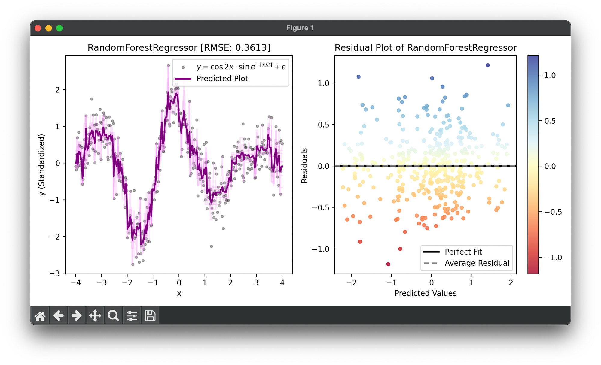
Test on the synthesized dataset of the curve $y=\cos{2x}\cdot\sin{e^{-\left\lceil x/2\right\rceil}}+\epsilon$:

from luma.ensemble.forest import RandomForestRegressor
from luma.preprocessing.scaler import StandardScaler
from luma.metric.regression import RootMeanSquaredError
from luma.visual.evaluation import ResidualPlot

import matplotlib.pyplot as plt
import numpy as np

np.random.seed(42)

X = np.linspace(-4, 4, 400).reshape(-1, 1)
y = (np.cos(2 * X) * np.sin(np.exp(-np.ceil(X / 2)))).flatten()
y += 0.2 * np.random.randn(400)

sc = StandardScaler()
y_trans = sc.fit_transform(y)

forest = RandomForestRegressor(n_trees=10,
                               max_depth=7,
                               bootstrap=True)

forest.fit(X, y_trans)

y_pred = forest.predict(X)
score = forest.score(X, y_trans, metric=RootMeanSquaredError)

fig = plt.figure(figsize=(10, 5))
ax1 = fig.add_subplot(1, 2, 1)
ax2 = fig.add_subplot(1, 2, 2)

ax1.scatter(X, y_trans, 
            s=10, c='black', alpha=0.3, 
            label=r'$y=\cos{2x}\cdot$' + \
                r'$\sin{e^{-\left\lceil x/2\right\rceil}}+\epsilon$')

for tree in forest.trees:
    ax1.plot(X, tree.predict(X), c='violet', alpha=0.2)

ax1.plot(X, y_pred, lw=2, c='purple', label='Predicted Plot')
ax1.legend(loc='upper right')
ax1.set_xlabel('x')
ax1.set_ylabel('y (Standardized)')
ax1.set_title(f'RandomForestRegressor [RMSE: {score:.4f}]')

res = ResidualPlot(forest, X, y_trans)
res.plot(ax=ax2)

plt.tight_layout()
plt.show()

Applications

• Real Estate: Predicting house prices based on features like location, size, and number of bedrooms.
• Finance: Estimating the future value of an investment based on historical data.
• Energy: Forecasting power consumption based on past consumption patterns and weather data.
• Healthcare: Predicting patient outcomes based on their medical histories and treatment plans.

Strengths and Limitations

Strengths

• Accuracy: Often provides high predictive accuracy that competes with the best supervised learning algorithms.
• Robustness: Handles outliers, missing values, and categorical features well.
• Versatility: Can be used for both regression and classification tasks.
• Feature Importance: Automatically ranks the importance of different features for the prediction.

Limitations

• Interpretability: The model's complex structure makes it hard to interpret compared to a single decision tree.
• Computationally Intensive: Requires more computational resources and time to train compared to other algorithms, especially as the number of trees increases.
• Overfitting with Noise: Can overfit datasets with a lot of noise.

Advanced Topics

• Hyperparameter Tuning: Adjusting the number of trees, max depth of the trees, min samples split, and min samples leaf can significantly impact the model's performance.
• Tree Ensemble Methods: Exploring other ensemble methods like Gradient Boosting and XGBoost for comparison with Random Forest.
• Handling Imbalanced Data: Techniques like SMOTE (Synthetic Minority Over-sampling Technique) can be integrated with Random Forest to handle imbalanced datasets effectively.

References

1. Breiman, Leo. "Random forests." Machine learning 45.1 (2001): 5-32.
2. Liaw, Andy, and Matthew Wiener. "Classification and regression by randomForest." R news 2.3 (2002): 18-22.