Voting Classifier

Introduction

The Voting Classifier is a machine learning model that combines the predictions from multiple different models to make a final prediction. This technique is a form of ensemble learning, where multiple models, often of different types, are strategically combined to improve prediction accuracy, robustness, and performance over any single model. Voting can be done in two ways: hard voting and soft voting.

Background and Theory

Ensemble methods like the Voting Classifier are based on the wisdom of crowds theory, which suggests that the collective prediction of a group of models is more accurate than that of a single model. The Voting Classifier aggregates the predictions of each base classifier and predicts the class that gets the most votes for hard voting, or the highest probability for soft voting, as the final prediction.

Mathematical Foundations

Let's consider a classification problem with $N$ classifiers $C_1, C_2, \ldots, C_N$ making predictions for a sample $x$. The final prediction $\hat{Y}$ can be formulated differently based on the voting strategy:

• Hard Voting: The predicted class label is the one with the majority votes from all classifiers.
  $\hat{Y}_{hard}(x) = mode\{C_1(x), C_2(x), ..., C_N(x)\}$
• Soft Voting: The predicted class label is the one with the highest sum of predicted probabilities from all classifiers. This requires all classifiers to be capable of predicting probabilities.
  $\hat{Y}_{soft}(x) = \arg\max \sum_{i=1}^{N} p_{i}(x)$
  where $p_{i}(x)$ is the predicted probability of the target class by the $i^\text{th}$ classifier.
  

Procedural Steps

1. Selection of Base Classifiers: Choose a diverse set of classifiers to be included in the ensemble. Diversity can be achieved through different algorithms, hyperparameters, or training subsets.
2. Training: Each base classifier is trained independently on the training data.
3. Voting:
   • In hard voting, each classifier votes for a single class, and the class with the majority votes is chosen as the final prediction.
   • In soft voting, each classifier provides probabilities for each class, and the class with the highest aggregated probability is chosen as the final prediction.
4. Final Prediction: Aggregate the predictions of all classifiers based on the chosen voting strategy to make the final prediction for each input sample.

Implementation

Parameters

• estimators: List[Estimator], default = None
  List of estimators to vote
  
• voting: Literal['label', 'prob'], default = ‘label’
  Voting criterion, ‘label’ for hard voting and ‘prob’ for soft voting
  
• weights: Vector[Scalar], default = None
  Weights for each classifier on voting
  

Examples

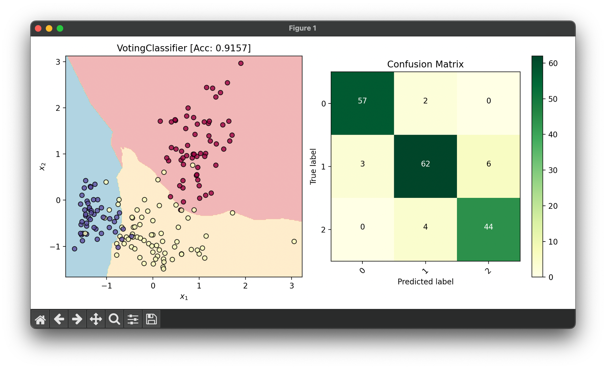
Test on the wine dataset with 7th and the last feature:

from luma.preprocessing.scaler import StandardScaler
from luma.model_selection.split import TrainTestSplit
from luma.classifier.neighbors import KNNClassifier
from luma.classifier.svm import KernelSVC
from luma.classifier.logistic import SoftmaxRegressor
from luma.ensemble.vote import VotingClassifier
from luma.visual.evaluation import DecisionRegion, ConfusionMatrix

from sklearn.datasets import load_wine
import matplotlib.pyplot as plt
import numpy as np

np.random.seed(42)

X, y = load_wine(return_X_y=True)
X = X[:, [6, -1]]

sc = StandardScaler()
X_std = sc.fit_transform(X)

X_train, X_test, y_train, y_test = TrainTestSplit(X_std, y, test_size=0.2).get
X_cat = np.concatenate((X_train, X_test))
y_cat = np.concatenate((y_train, y_test))

estimators = [
    KNNClassifier(n_neighbors=5),
    KernelSVC(C=1.0, gamma=1.0, kernel='rbf'),
    SoftmaxRegressor(learning_rate=0.01, regularization='l2')
]

vote = VotingClassifier(estimators=estimators, voting='label')
vote.fit(X_train, y_train)

score = vote.score(X_cat, y_cat)

fig = plt.figure(figsize=(10, 5))
ax1 = fig.add_subplot(1, 2, 1)
ax2 = fig.add_subplot(1, 2, 2)

dec = DecisionRegion(vote, X_cat, y_cat, 
                     cmap='Spectral', 
                     title=f'{type(vote).__name__} [Acc: {score:.4f}]')
dec.plot(ax=ax1)

conf = ConfusionMatrix(y_cat, vote.predict(X_cat), cmap='YlGn')
conf.plot(ax=ax2, show=True)

Applications

• Political Science: Predicting election outcomes based on different polls and models.
• Medical Diagnosis: Combining different diagnostic models to improve the accuracy of patient diagnoses.
• Customer Sentiment Analysis: Aggregating predictions from different sentiment analysis models to determine overall customer sentiment towards a product or service.
• Financial Forecasting: Integrating diverse financial models to predict stock prices or market movements more accurately.

Strengths and Limitations

Strengths

• Improved Accuracy: Often achieves higher accuracy than individual classifiers by leveraging their diverse strengths.
• Reduced Overfitting: By combining multiple models, it tends to generalize better, reducing the risk of overfitting.
• Flexibility: Works with any type of classifier, regardless of the algorithm.

Limitations

• Increased Complexity: More complex to implement and manage compared to single models.
• Computationally Demanding: Requires more computational resources since multiple classifiers need to be trained and stored.
• Interpretability: The final decision-making process is less transparent due to the involvement of multiple classifiers.

Advanced Topics

• Weighted Voting: Assigning different weights to the votes of each classifier, based on their performance, to further improve the accuracy.
• Model Diversity: Exploring strategies for selecting a diverse set of classifiers to maximize the ensemble's performance.
• Dynamic Voting: Adjusting the voting strategy or classifier weights based on the performance of the ensemble on a validation set during training.

References

1. Kuncheva, Ludmila I. "Combining pattern classifiers: methods and algorithms." John Wiley & Sons, 2014.
2. Polikar, Robi. "Ensemble based systems in decision making." IEEE Circuits and Systems Magazine 6.3 (2006): 21-45.