Stacking Classifier

Introduction

Stacking (short for stacked generalization) involves training a model to combine the predictions of several other models. The aim is to use the stacked model to achieve better predictive performance than any single model in the ensemble. Cross-validation (CV) is often employed in stacking to mitigate the risk of overfitting, especially when training the meta-learner (the model that combines the predictions of the base learners).

Background and Theory

Stacking typically involves two levels of learners: base learners and a meta-learner. The base learners are trained on the original training data, and their predictions (for each data point in the training set) are used as features to train the meta-learner. The meta-learner's job is to learn how to best combine the base learners' predictions into a final prediction.

Cross-validation adds an extra layer of robustness by ensuring that the meta-learner is not trained on the same data used to train the base learners, thereby reducing the risk of overfitting. This is usually achieved by splitting the training data into several folds. For each fold, the base models are trained on the other folds and make predictions on the current fold. These predictions are then used as features for training the meta-learner.

Mathematical Foundations

Let's consider a dataset with $n$ samples and $m$ features, represented as $(x_i, y_i)$ for $i=1, \ldots, n$, where $x_i$ is the feature vector of the $i$-th sample and $y_i$ is its corresponding target. In stacking, the dataset is divided into $k$ folds for cross-validation. For each fold $j$, the base models are trained on all data except the data in fold $j$ and then predict the outcomes for fold $j$. This process is mathematically represented as:

1. For each fold $j = 1, \ldots, k$:
   • Train each base model $l$ on $\{(x_i, y_i) | i \notin \text{fold } j\}$
   • Predict $\hat{y}_{i}^{l}$ for $i$ in fold $j$ using model $l$
2. Train the meta-model on $\{(\hat{y}_{i}^{1}, \ldots, \hat{y}_{i}^{L}, y_i) | i = 1, \ldots, n\}$, where $L$ is the number of base models.

This approach ensures that the predictions $\hat{y}_{i}^{l}$, which are used as features for the meta-model, are always generated from models that were not trained on the part of the data they are making predictions for.

Procedural Steps

1. Split the Data: Divide the training data into $k$ folds for cross-validation.
2. Train Base Models: For each fold, train each base model on the data excluding that fold.
3. Generate Base Predictions: Use the trained base models to predict the outcomes for the data in the excluded fold. This forms a new dataset where the features are the predictions of the base models.
4. Train Meta-Model: Use the dataset generated in the previous step to train the meta-model. The target values remain the same as in the original dataset.
5. Final Prediction: To make predictions on new data, first use the base models to generate predictions, then feed these predictions into the meta-model to obtain the final prediction.

Implementation

Parameters

• estimators: List[Estimator]
  List of base estimators
  
• final_estimator: Estimator, default = SoftmaxRegressor()
  Final meta-estimator
  
• pass_original: bool, default = False
  Whether to pass the original data to final estimator
  
• drop_threshold: float, default = None
  Omitting threshold for base estimators (None not to omit any estimators)
  
• method: Literal['pred', 'prob'], default = ‘pred’
  Methods called for each base estimator
  
• cv: int, default = 5
  Number of folds for cross-validation
  
• fold_type: FoldType, default = KFold
  Fold type
  
• shuffle: bool, default = True
  Whether to shuffle the dataset when cross-validating
  
• random_state: int, default = None
  Seed for random splitting
  
• **kwargs: Dict[str, Any]
  Additional parameters for final estimator (i.e. learning_rate)
  

Examples

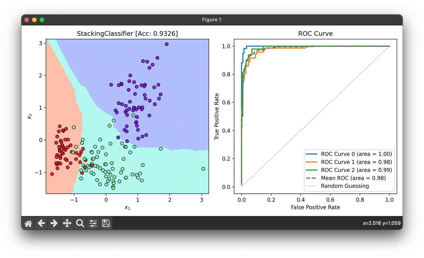
Test on reduced wine dataset transformed into $\mathbb{R}^5$ space:

from luma.ensemble.stack import StackingClassifier
from luma.classifier.discriminant import LDAClassifier
from luma.classifier.logistic import SoftmaxRegressor
from luma.classifier.naive_bayes import GaussianNaiveBayes
from luma.classifier.neighbors import KNNClassifier
from luma.classifier.tree import DecisionTreeClassifier
from luma.preprocessing.scaler import StandardScaler
from luma.model_selection.split import TrainTestSplit
from luma.model_selection.fold import StratifiedKFold
from luma.visual.evaluation import DecisionRegion, ROCCurve

from sklearn.datasets import load_wine
import matplotlib.pyplot as plt
import numpy as np

np.random.seed(42)

X, y = load_wine(return_X_y=True)
X = X[:, [6, -1]]

sc = StandardScaler()
X_std = sc.fit_transform(X)

X_train, X_test, y_train, y_test = TrainTestSplit(X_std, y,
                                                  test_size=0.3,
                                                  stratify=True).get

estimators = [
    LDAClassifier(),
    GaussianNaiveBayes(),
    SoftmaxRegressor(learning_rate=0.01, alpha=0.01, regularization='l2'),
    KNNClassifier(n_neighbors=5),
    DecisionTreeClassifier(max_depth=10, criterion='gini')
]

stack = StackingClassifier(estimators=estimators,
                           pass_original=False,
                           drop_threshold=0.5,
                           method='prob',
                           cv=5,
                           fold_type=StratifiedKFold,
                           regularization='l1',
                           shuffle=True,
                           verbose=True)

stack.fit(X_train, y_train)

X_all = np.vstack((X_train, X_test))
y_all = np.hstack((y_train, y_test))

score = stack.score(X_all, y_all)

fig = plt.figure(figsize=(10, 5))
ax1 = fig.add_subplot(1, 2, 1)
ax2 = fig.add_subplot(1, 2, 2)

dec = DecisionRegion(stack, X_all, y_all, 
                     title=f'{type(stack).__name__} [Acc: {score:.4f}]')
dec.plot(ax=ax1)

roc = ROCCurve(y_all, stack.predict_proba(X_all))
roc.plot(ax=ax2, show=True)

Applications

• Competitive Machine Learning: Stacking is popular in machine learning competitions, where slight improvements in predictive accuracy can be crucial.
• Regression Problems: Stacking can combine regression models to predict continuous outcomes.
• Classification Problems: It is also effective in classification, combining different classifiers' decisions.

Strengths and Limitations

Strengths

• Improved Accuracy: By combining multiple models, stacking can often achieve higher accuracy than any single model.
• Model Diversity: Stacking can leverage the strengths of various models, making it versatile across different types of data and tasks.

Limitations

• Complexity: Stacking can be more complex and time-consuming to implement and train than simpler models.
• Risk of Overfitting: While cross-validation helps, there's still a risk of overfitting, especially with a large number of base models or a complex meta-learner.

Advanced Topics

• Feature Engineering for Meta-Learner: Beyond using just the predictions of base models, incorporating original features or engineered features can sometimes improve performance.
• Dynamic Stacking: Techniques that adaptively select models or adjust weights based on performance can further enhance stacking strategies.

References

1. Wolpert, David H. "Stacked generalization." Neural networks 5.2 (1992): 241-259.
2. Breiman, Leo. "Stacked regressions." Machine learning 24.1 (1996): 49-64.