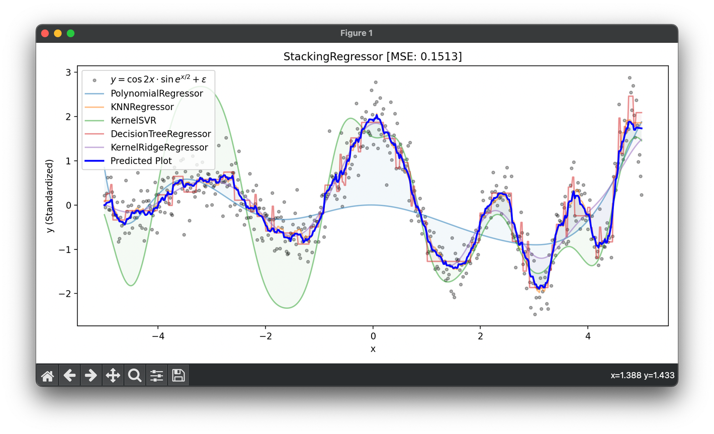
Stacking Regressor

Introduction

Stacking Regressor is an ensemble learning technique that combines multiple regression models via a meta-regressor. The base level models are trained based on the complete training set, then the meta-regressor is fitted based on the outputs—predictions of these base models. The goal is to blend different regression models to improve the overall prediction accuracy compared to any single model in the ensemble.

Background and Theory

Stacking involves two or more base regressors and a meta-regressor. The base regressors are individual models that learn to predict the target variable. The meta-regressor then learns how to best combine these predictions into a final prediction. This approach leverages the strengths and mitigates the weaknesses of individual models.

Mathematical Foundations

Let $\{(x_i, y_i)\}_{i=1}^{N}$ be a training set of $N$ samples, where $x_i$ is the $i^\text{th}$ feature vector, and $y_i$ is the corresponding target value. Suppose we have $M$ base regressors, $f_1, f_2, \ldots, f_M$. The stacking regressor works in two main steps:

1. Base Regressors Training:
   Each base regressor $f_m$ is trained on the training set, and its predictions $\hat{y}_{i}^{m}$ for each sample $x_i$ are obtained.
2. Meta-Regressor Training:
   The meta-regressor is trained on a new dataset constructed from the predictions of the base regressors, where the feature vector for each sample $i$ is $[\hat{y}_{i}^{1}, \hat{y}_{i}^{2}, \ldots, \hat{y}_{i}^{M}]$, and the target is the true values $y_i$.

The final prediction for a new sample $x$ is obtained by first predicting with the base regressors to get $\hat{y}^{m}$, then inputting $[\hat{y}^{1}, \hat{y}^{2}, \ldots, \hat{y}^{M}]$ into the meta-regressor to get the final prediction $\hat{y}$.

Procedural Steps

1. Train Base Regressors:
   Train each base regressor on the full training dataset.
2. Predict with Base Regressors:
   Use the trained base regressors to predict the target for both the training set and (optionally) for validation/test sets.
3. Train Meta-Regressor:
   Create a new training set where each input feature is the prediction of one base regressor from the previous step. Train the meta-regressor on this new dataset.
4. Final Prediction:
   To predict the target for a new instance, first predict with all base regressors, then use these predictions as input features for the meta-regressor to obtain the final prediction.

Implementation

Parameters

• estimators: List[Estimator]
  List of base estimators
  
• final_estimator: Estimator, default = LinearRegressor()
  Final meta-estimator
  
• pass_original: bool, default = False
  Whether to pass the original data to final estimator
  
• cv: int, default = 5
  Number of folds for cross-validation
  
• fold_type: FoldType, default = KFold
  Fold type
  
• shuffle: bool, default = True
  Whether to shuffle the dataset when cross-validating
  
• random_state: int, default = None
  Seed for random splitting
  
• **kwargs: Dict[str, Any]
  Additional parameters for final estimator
  

Examples

Test on the synthesized dataset of the curve $y=\cos(2x)\cdot\sin{e^{x/2}}+\epsilon$:

from luma.ensemble.stack import StackingRegressor
from luma.regressor.neighbors import KNNRegressor
from luma.regressor.svm import KernelSVR
from luma.regressor.tree import DecisionTreeRegressor
from luma.regressor.poly import PolynomialRegressor
from luma.regressor.linear import KernelRidgeRegressor
from luma.preprocessing.scaler import StandardScaler
from luma.metric.regression import MeanSquaredError

import matplotlib.pyplot as plt
import numpy as np

np.random.seed(42)

X = np.linspace(-5, 5, 500).reshape(-1, 1)
y = (np.cos(2 * X) * np.sin(np.exp(X / 2))).flatten()
y += 0.2 * np.random.randn(500)

sc = StandardScaler()
y_trans = sc.fit_transform(y)

estimators = [
    PolynomialRegressor(deg=9, alpha=0.01, regularization='l2'),
    KNNRegressor(n_neighbors=10), 
    KernelSVR(C=1.0, gamma=3.0, kernel='rbf'),
    DecisionTreeRegressor(max_depth=7, random_state=42),
    KernelRidgeRegressor(alpha=1.0, gamma=1.0, kernel='rbf')
]

stack = StackingRegressor(estimators=estimators,
                          pass_original=False,
                          cv=5,
                          shuffle=True,
                          verbose=True)

stack.fit(X, y_trans)

y_pred = stack.predict(X)
score = stack.score(X, y_trans, metric=MeanSquaredError)

fig = plt.figure(figsize=(10, 5))
plt.scatter(X, y_trans, 
            s=10, c='black', alpha=0.3, 
            label=r'$y=\cos{2x}\cdot\sin{e^{x/2}}+\epsilon$')

for est in stack:
    est_pred = est.predict(X)
    plt.plot(X, est_pred, 
             alpha=0.5, label=f'{type(est).__name__}')
    plt.fill_between(X.flatten(), est_pred, y_pred, alpha=0.05)

plt.plot(X, y_pred, lw=2, c='blue', label='Predicted Plot')
plt.legend()
plt.xlabel('x')
plt.ylabel('y (Standardized)')
plt.title(f'StackingRegressor [MSE: {score:.4f}]')

plt.tight_layout()
plt.show()

Applications

• Real Estate Price Prediction: Combining various models to improve accuracy in predicting house prices based on features like location, size, and amenities.
• Financial Forecasting: Using stacking to predict stock prices or economic indicators by blending different types of models.
• Energy Consumption Forecasting: Improving predictions of energy demand in buildings or regions by stacking models that consider weather conditions, time factors, and historical consumption data.

Strengths and Limitations

Strengths

• Improved Accuracy: Stacking often achieves better performance than any single model by effectively combining their predictions.
• Model Diversity: Can leverage the unique strengths of different regression models, providing a versatile approach to various regression tasks.

Limitations

• Complexity: Implementing and tuning a stacking regressor can be more complex than working with individual models.
• Overfitting Risk: If not properly validated, stacking can overfit the training data, especially with complex base models or meta-regressors.

Advanced Topics

• Cross-Validated Stacking: Using cross-validation to train base models and generate out-of-sample predictions for training the meta-regressor, reducing overfitting.
• Feature Engineering in Stacking: In addition to using predictions from base models, incorporating original features or new engineered features in the meta-regressor training can enhance the stacking model's performance.

References

1. Breiman, Leo. "Stacked regressions." Machine learning 24.1 (1996): 49-64.
2. Wolpert, David H. "Stacked generalization." Neural networks 5.2 (1992): 241-259.